Contents
- Intro
- Disclaimer
- Metrology concepts
- SI volt history
- SI resistance history
- Today’s technology
- Practical experiment theory
- DCV Source reference setup
- Calibration targets
- Experiment execution
- Error budget
- Conclusion
Intro
Every measurement need a known reference point. How do we know that one second is really a second? How do we know that one meter is indeed 1 meter, not 990 mm or 1010 mm? Science about measurements is called metrology. This is important aspect of any engineering application, be it electronics, machining, analytics and even biology and chemistry. Because of this science we can be sure, that ruler from shop in USA and ruler from shop in Europe or Asia is same. Same applies to electric measurements, such as voltage, current, frequency and resistance.
Disclaimer
Redistribution and use of this article or any part of it, including images or files referenced in it, in source and binary forms, with or without modification, are permitted provided that the following conditions are met:
- Redistributions of article must retain the above copyright notice, this list of conditions, link to this page (https://xdevs.com/article/volt_xfer/) and the following disclaimer.
- Redistributions of files in binary form must reproduce the above copyright notice, this list of conditions, link to this page (https://xdevs.com/article/volt_xfer/), and the following disclaimer in the documentation and/or other materials provided with the distribution, for example Readme file.
All information posted here is hosted just for education purposes and provided AS IS. In no event shall the author, xDevs.com site, or any other 3rd party be liable for any special, direct, indirect, or consequential damages or any damages whatsoever resulting from loss of use, data or profits, whether in an action of contract, negligence or other tortuous action, arising out of or in connection with the use or performance of information published here.
If you willing to contribute or have interesting documentation to share regarding measurements or metrology and electronics in general, you can do so by following these simple instructions.
Metrology concepts
Measurements of any physical quantity or value can never be exact. One can only know its value with a range of uncertainty. If measurement provides some quantity A, the measurement is written with an uncertainty: A ± ΔA. This expresses that the actual value of A is somewhere between A – ΔA and A + ΔA.
Resolution, precision and accuracy
Let’s go some precision hunting. Some might confuse measurement resolution, precision and accuracy. These concepts are actually different things and can be measured and expressed independently.
Accuracy – difference between the measurement result and true value of the signal, or in other words, closeness of agreement between a measured quantity value and a true quantity value of a measurand.
Precision – closeness of agreement between indications or measured quantity values obtained by replicate measurements on the same or similar objects under same specified conditions. High precision system will provide same results every time the measurement on constant input signal is taken.
Resolution – smallest detectable change in measurement result, that cause perceptible change in output value. Resolution is often provided in bits. Ideal 1-bit ADC will generate “1” when input analog signal larger than 50% of the range, and “0” if less. ADC with 8 bits of resolution have 28 = 256 steps (from 00000000 to 11111111), thus able to detect 100% / 256 = 0.390625% change of the range. If range limited between 0.0V and 10.0V input, then such ADC can resolve input analog voltage with 39.0625 mVDC step per 1 bit of digital code output. As result we say this ADC have 8 bits of resolution.
Higher resolution does not provide better accuracy or precision, it only provides smaller value step size. Noise and other system errors reduce actual useful resolution. Together with input signal range resolution provide sensitivity of the ADC.
Imagine yourself shooting a target with arrows. One hit is one measurement sample. If we take just one sample, we cannot know how accurate is it. But if we make a series of samples, we can see much more.
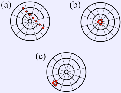
On target case a we have low precision and low accuracy, with shots all over the place. We cannot clearly see what is real value. Need improve both precision and accuracy to get sample hits like on target b. This is high precision with high accuracy. Now if we still use high precision, but our accuracy is low, we will get target image c. That’s why calibration even more important for high-precision equipment, as even if we have high precision, it does not automatically get good accuracy as well without calibration.
There is one more case missing on targets above – with low precision, and high accuracy. If you got concept right, you should know how it should look like, and feel free to share your thought in comments!
SI volt history
The volt is the derived unit for electric potential, electric potential difference (voltage), and EMF. The volt is named in honour of the Alessandro Volta, who invented the voltaic pile, possibly the first chemical battery. History of electrical values. Currently 1 Volt is defined as the difference in electric potential between two points of a conducting wire when an electric current of one ampere dissipates one watt of power between those points, however this definition will be adjusted by upcoming SI redefinition in 2019.
Today’s technology
The Josephson Voltage Standard
Josephson effect is a super conducting physical phenomenon that relates voltage to frequency through the ratio of fundamental constants. It was discovered in 1962, by 22-year old Brian D. Josephson. A Josephson array, using multiple of superconductor-insulator-superconductor junctions form the integrated circuit. In superconducting state, when exposed to RF radiation, the dc voltage VJ across the junction will be formed and only discrete values (“steps”) will be generated. This provide an intrinsic, independently reproducible standard that is used to represent rather than realize the SI volt. The output voltage of a single Josephson junction is defined as:
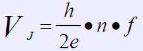
- VJ = Junction voltage
- ƒ = Frequency in GHz
- e = elementary charge (1.60217662 × 10⁻¹⁹ coulombs)
- h = Planck’s constant (6.62607004 × 10⁻³⁴ m2 kg/s)
- n = a positive or negative integer
Today h/2e is called Josephson constant, KJ-90, which is defined as 483597.9 GHz/V without any uncertainty. By means of Josephson junctions, voltage can be reproduced with relative uncertainties of less than one part in ten billion (1 : 1010, i.e. 1 nV at 10 V). Since we already have achieved much better uncertainty at 10-16 levels for frequency, and rest of parameters in formula are physics constants, voltage standards based on Josephson arrays today are widely used as national Volt standard worldwide.
Example voltage standard system using this effect is one developed by PTB in Germany. This system consists of a 75 GHz Gunn-oscillator, locked by a PLL to a Fluke 910R, a GPS-controlled Rhubidium Frequency Standard. During operation, the probe with JJA circuit is immersed in a 42 litre dewar vessel with liquid helium to maintain constant temperature at ~4.2K. For chosen frequency of 75 GHz, the voltage difference between adjacent steps is about 155 μV. There are also other JJA systems that use other RF frequencies.
AC quantum voltmeter JJA-based voltmeter system with accuracy ±0.001ppm at 10VDC and 0.2ppm at 20VACpk-pk 1kHz.
The Quantum Hall Resistance Standard
The Quantum Hall effect provides a universal standard for electrical resistance that is theoretically based on only the Planck constant h and the electron charge e. Currently, this standard is implemented in GaAs/AlGaAs structures. In particular, the Hall resistance level can be accurately quantized to within 1 × 10⁻⁹ over a wide range of magnetic flux density, from 10 T down to 3.5 T, at a temperature of up to few K. The Quantum Hall effect comprises the quantization of the Hall resistance in two-dimensional electron systems in rational fractions of RK = = 25,812.807557(18) Ω, the resistance quantum level.
Despite 30 years of research into the Quantum Hall effect, the level of precision necessary for metrology, which is few ppb, has been achieved only in silicon and III-V heterostructure type devices. There are also new designs and development to implement QHR using graphene, such as this study.
Practical experiment theory
But all this marvelous physics science and related gear is not accesible for average hobbyist level, so next best solution would be using good solid-state references (SSR) with frequent cross-comparison between known calibrated standards for DC voltage, and precision stable resistance wirewound standards for resistance. And best candidate for such a DC Voltage source device would be Linear LTZ1000-based ultra-zener reference module (or newer 10V variant), to provide very stable and low-noise output. Size of final assembly can be kept small, allowing cheap shipping overseas and project cost while bit high (300-350$ in parts) is still within reach of any serious volt-nut.
Most accurate piece of voltage source/measurement gear I had during this experiment timeframe was old repaired Keithley 2001 7½-digit DMM, later calibrated by Tektronix in February 2014. Uncertainty of Tektronix calibration facility for 10V in Taiwan is ± 20 ppm. This accuracy level is not suitable for proper HP 3458A calibration. Even if my 2001 still stay precisely spot on with calibration, it’s own readings accuracy is 7+4ppm for 24 hours, with ADC’s linearity 2 ppm max.
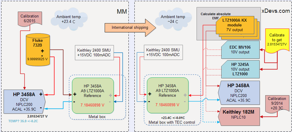
This experiment is alternative attempt to “import” calibration from known stable source, Fluke 732B, located in USA into my own home-lab, here in Taiwan. To perform this task, best solid-state reference will be used, Linear LTZ1000A, in form of HP 3458A’s opt-002 voltage reference A9 module. This reference module specified to be stable within 4 ppm/year window.
Idea is simple: get absolute voltage output of LTZ module, using Fluke 732B and calibrated HP 3458A as null-meter. This will allow to get voltage reading with 2ppm accuracy. Second step would be sending this LTZ module overseas using airmail to here.
Then I will use my 10V sources and my calibrated Keithley 182M nV-meter to calibrate my 10V sources, to get exactly same voltage difference, as we got with Fluke732B-LTZ. LTZ module temperature will be matched to ambient temperature with ±0.01°C tolerance. This is assuming that voltage output of LTZ itself did not change from shipping and stress.
Then HP 3458A would be calibrated using adjusted 10V sources, to import volt into it’s own reference. If everything goes well, direct reading of LTZ1000 module should then match expected 7.1846089 V.
Also transfer LTZ1000A voltage would be compared to three other LTZ1000-based modules, to get absolute voltage delta of those as well, using HP 3458A or K182M as null-meter. This, and monitoring in future would allow us to ensure that all four LTZ units stay stable over time.
Keysight USA (Loveland) calibration facility uncertainties
Keysight Malaysia (Penang) calibration facility uncertainties
DCV Source reference setup
Known voltage source is provided by one of our readers, precision enthusiast located in USA. Recently calibrated HP 3458A was used together with uncalibrated Fluke 732B as primary standard.
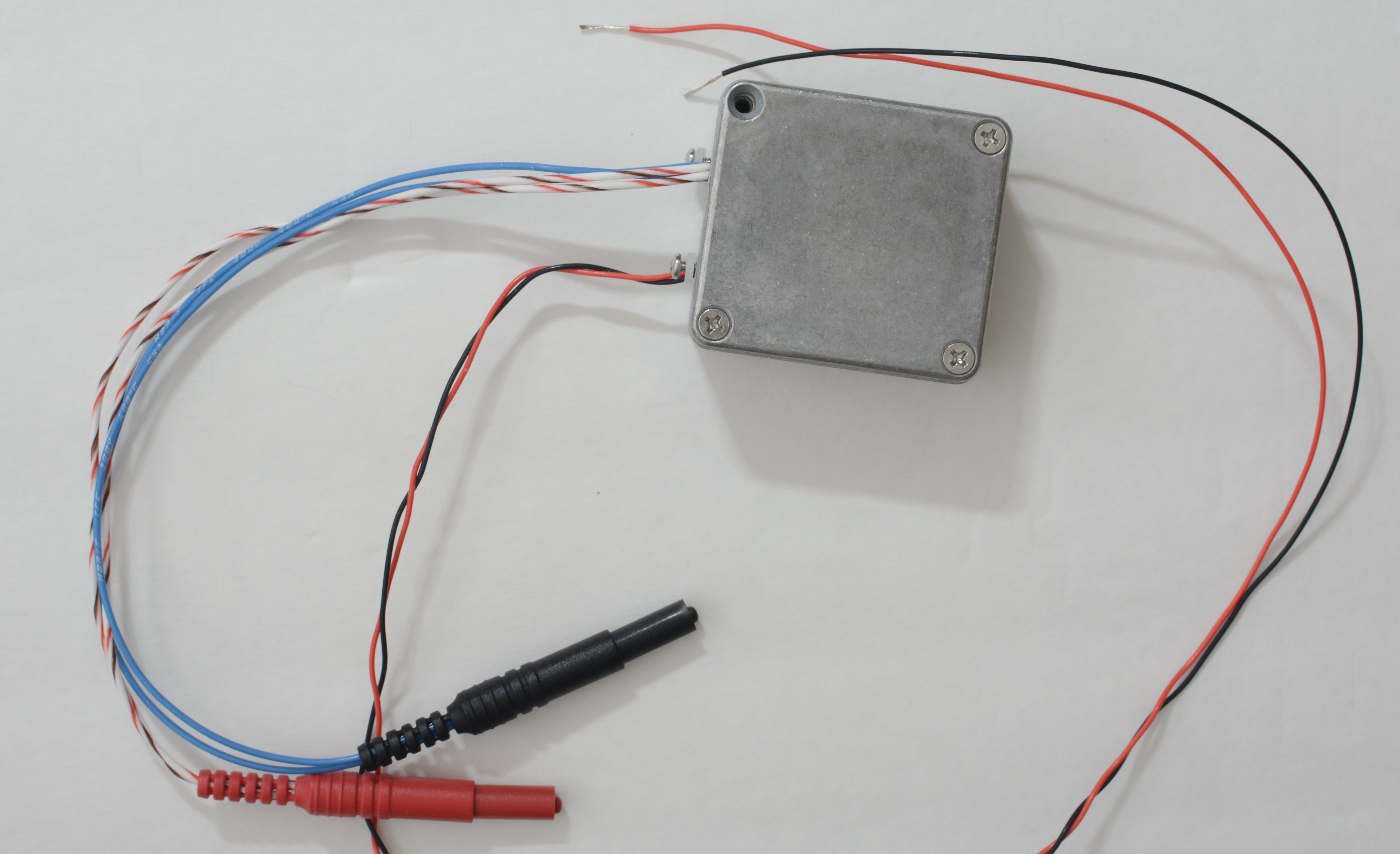
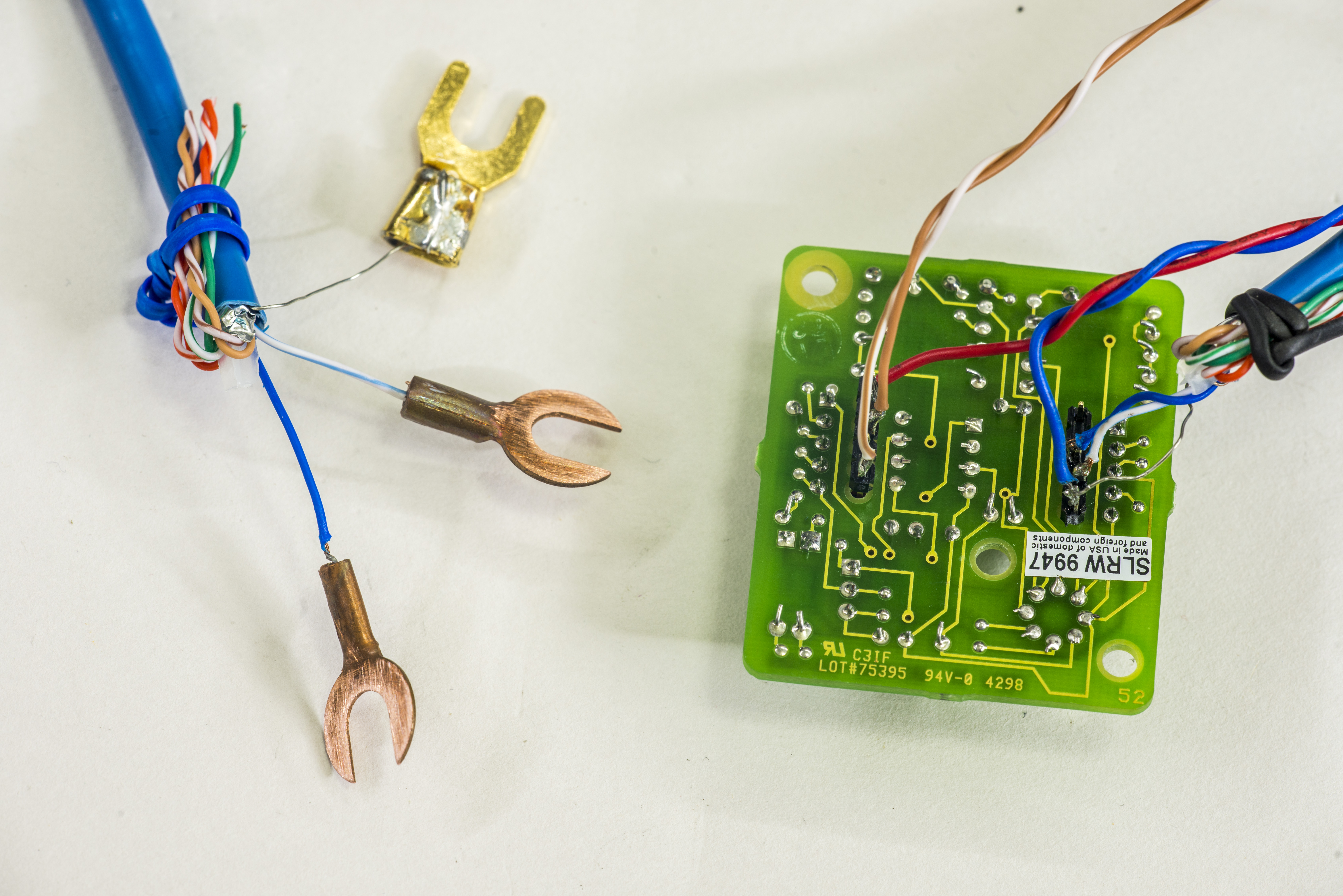
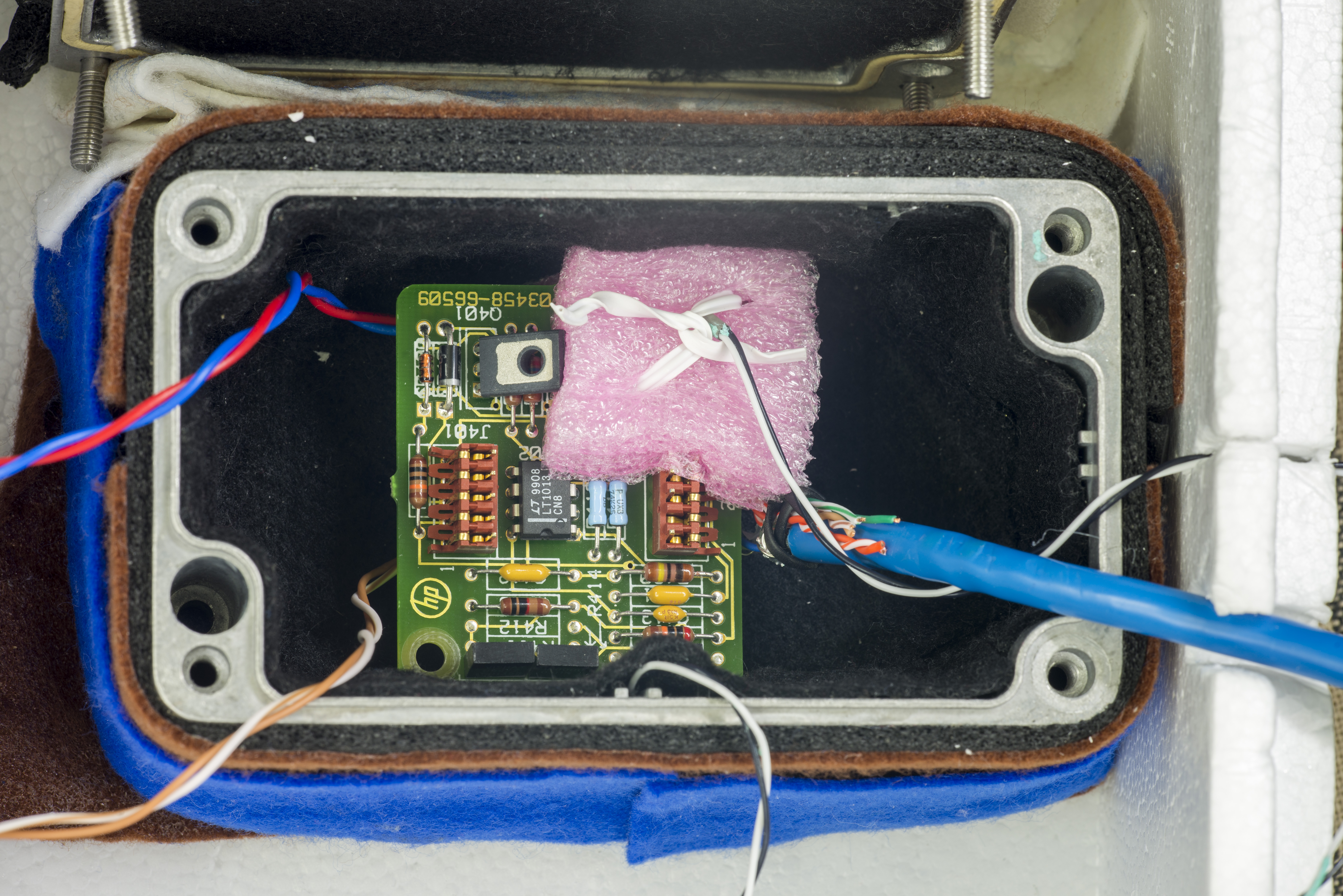
Here’s our voltage transfer module, HP 03458-66509 A9 PCBA module. This module is designed for use in 8ppm/year stable HP 3458A DMM. It is almost exact copy of Linear LTZ1000 reference schematics, with use of three Vishay Precision Group metal foil resistors and providing direct 7V zener output.

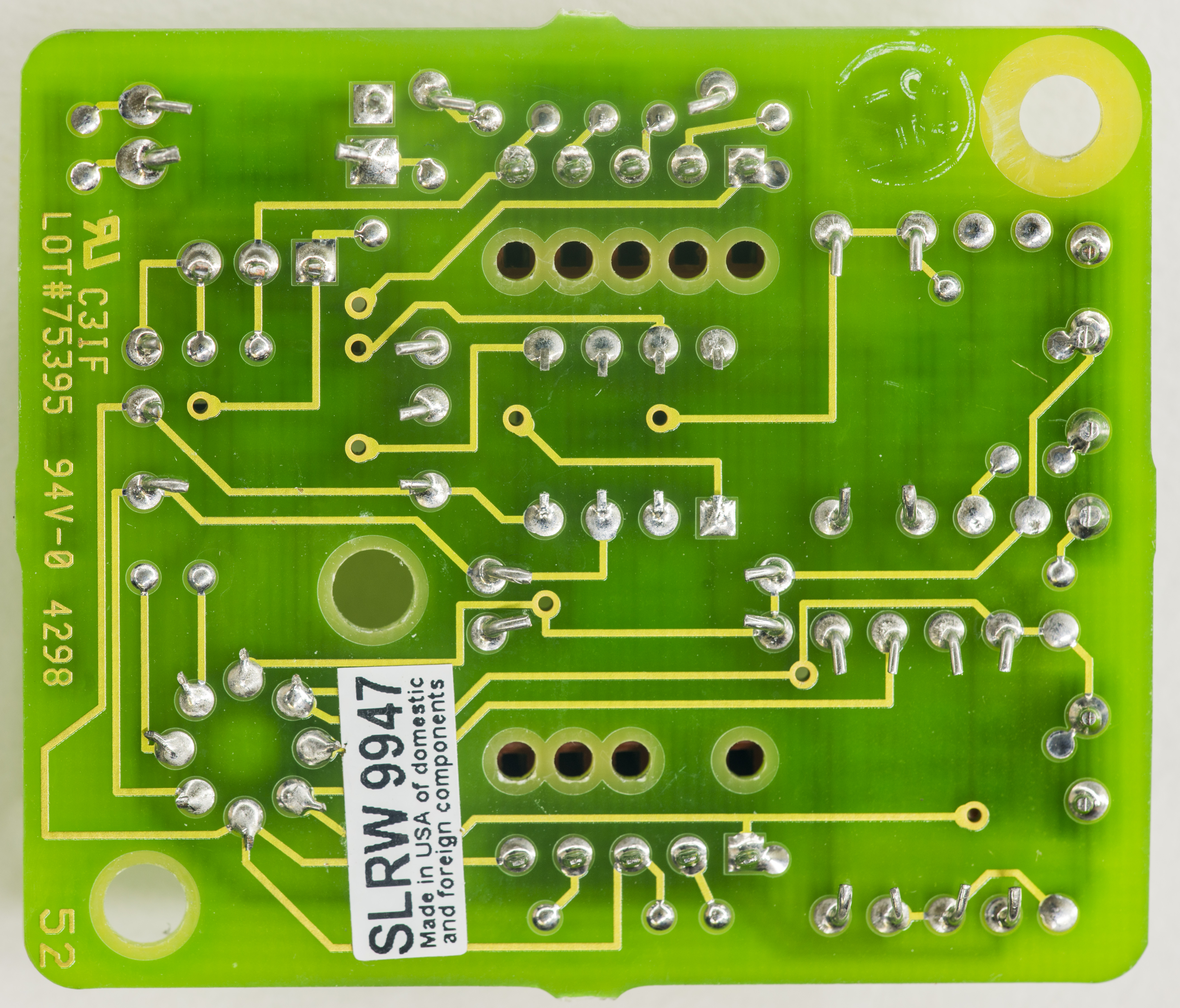

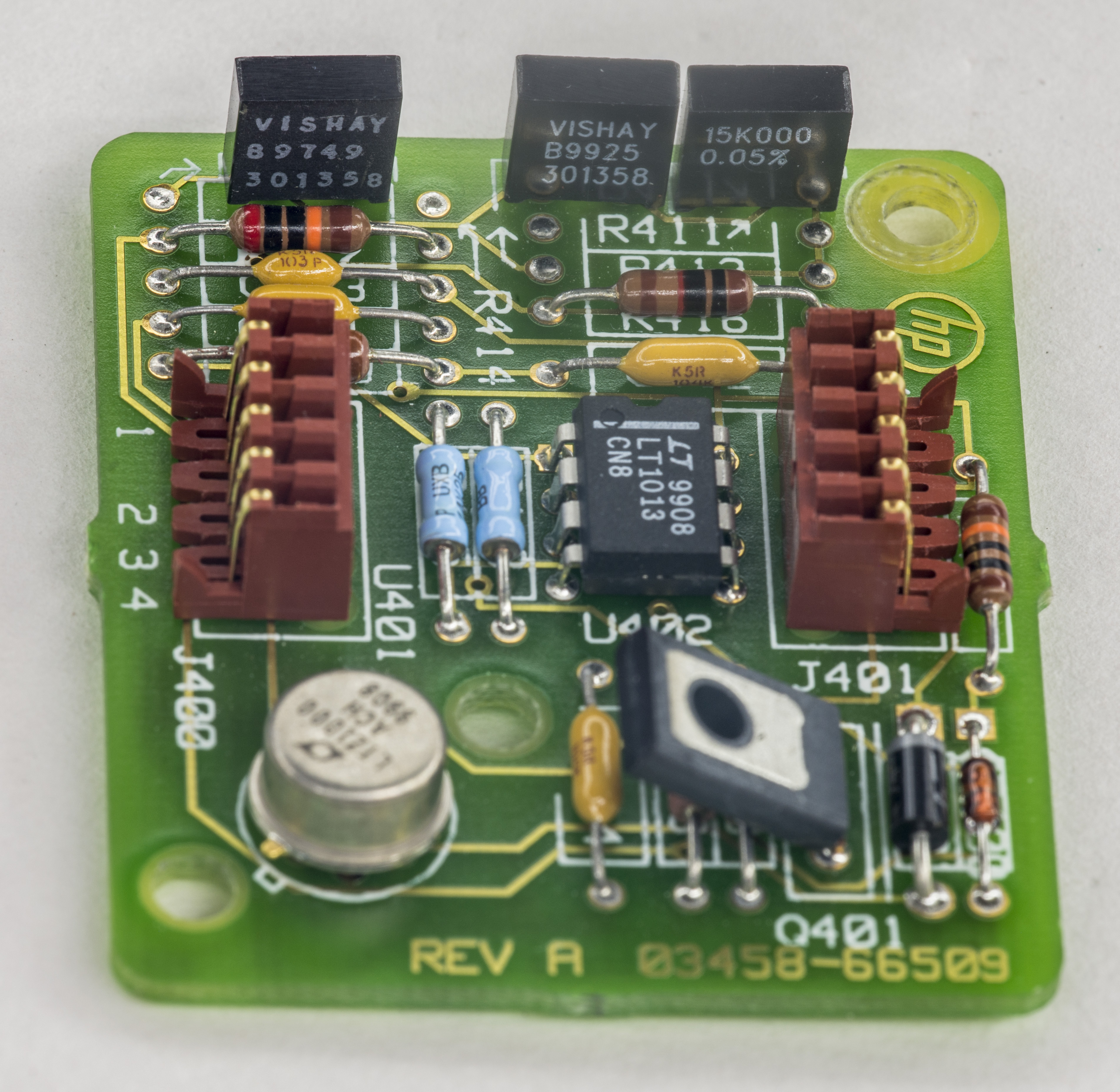
Module was installed in metal cast box to provide some shielding and isolate module itself from ambient airflow. Box was covered with some rags and located at one of 3458A’s.
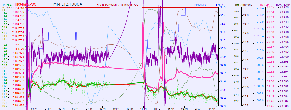
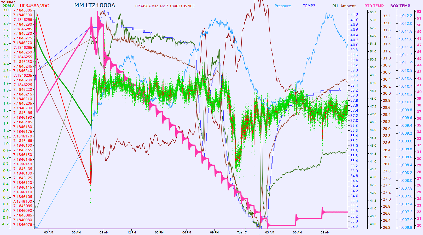
Datalog with LTZ data
Datalog with REF data
Initial TC estimation is -0.603ppm/K.
Experiment execution
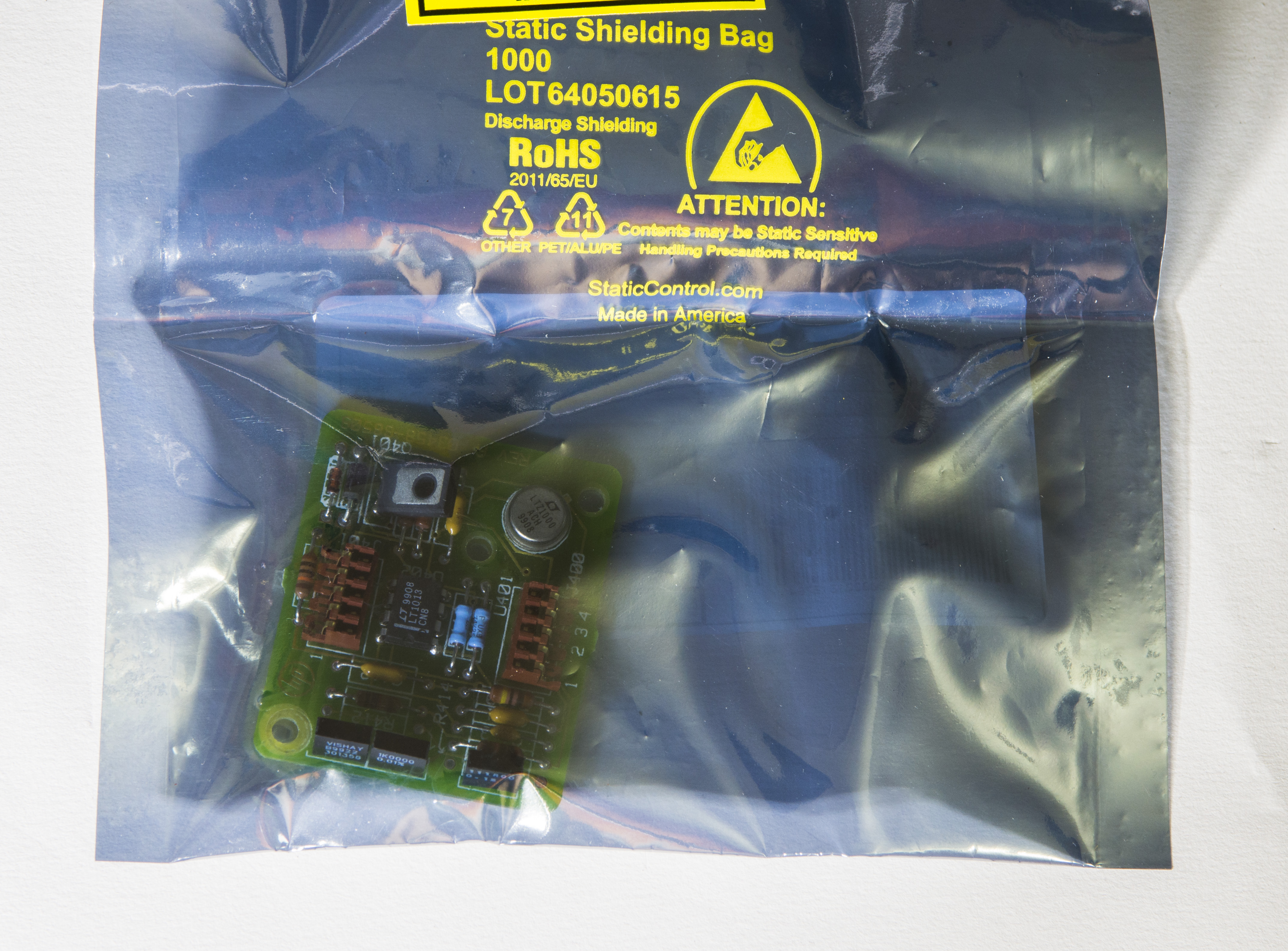
LTZ PCBA shipped from source location February 28, 2016 by regular USPS envelope mail.
Regular mail with hard packet and usual ESD bag was used for reference module, nothing fancy at all. LTZ PCBA received at destination location March 17, 2016, which makes 19 days in travel. This is a serious stretch for most of battery operated LTZ1000-based SSR’s if shipped hot (powered). Even if faster FedEx or DHL service used, travel time for international USA-Taiwan package would be still close to 6-8 days.
I prepared connector jig to avoid soldering and thermal stress on reference module, using common 0.1” pin header and Ethernet UTP CAT6 shielded cable. Heater and reference supply was routed by two separate wires to Keithley 2400, configured for +15.000V source with 105mA current compliance. Copper spade lugs are used to ensure low thermal EMF. They were cleaned with sandpaper right before connecting to DMM’s binding posts, to prevent copper oxide from ruining accuracy.

Reference module installed in metal cast box with insulation layers to have smooth and controlled temperature environment. Bottom surface of metal box is attached to 55W TEC module, which is cooled by external fansink. Reference box is further enclosed in styrofoam box with 10mm walls to reduce environment impact and allow better temperature regulation.
Black/white twisted cable is from Honeywell HEL-705 platinum 1KΩ RTD. One is fixed on metal wall, routed to temperature sense input on Keithley 2510 as feedback. Second is fixed on foam box right above the LTZ1000A zener IC, and routed to Keithley 2002 for relative temperature measurement.
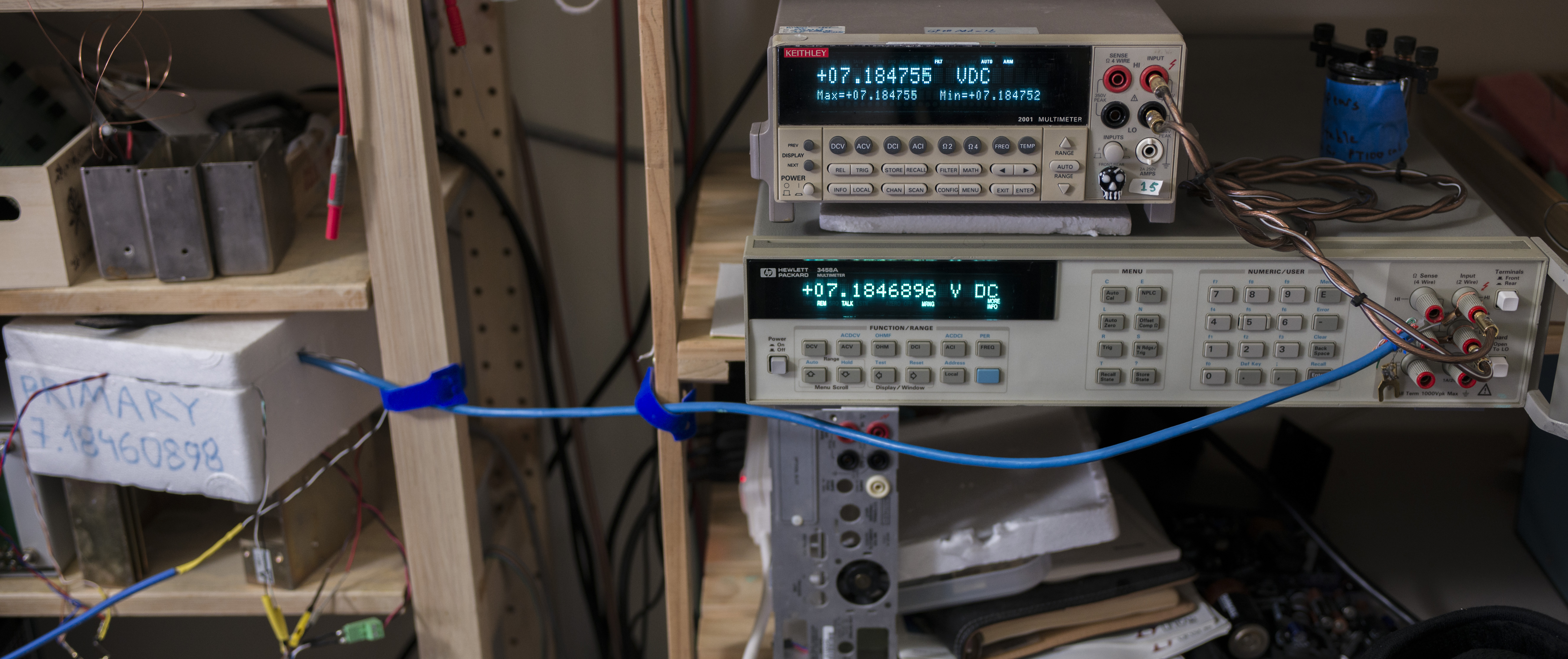
Temperature controlled by precision TEC SMU, Keithley 2510 which is well able to maintain temperatures within 0.01°C on this setup. This arrangement was tested multiple times before and allow to control temperatures in range from +18°C to +60°C with ease. After everything set, reference output is connected to HP 3458A for initial direct measurements:

Initial datalog started:
Keithley 2001 used as old standard hooked in parallel as well:
Since now we know exact transfer voltage reference at +23.4°C temperature, first easy step is to check absolute accuracy of DMMs I already have here.
| Instrument under test | Reading/compare | Error, ppm/REF | Conditions | Last calibrated |
|---|---|---|---|---|
| Keithley 2001 | 7.184756 | +20.46 | Warmup 24 hours | February 2014 by Tektronix |
| Keithley 2002 #1 | Warmup 24 hours | 2007 | ||
| Keithley 2002 #2 | Warmup 24 hours | 2012 | ||
| Keithley 182-M | Warmup 24 hours | 2015 | ||
| HP 3458A | 7.18469035 | +11.32 | Run 24/7 last 2 months | January 2016, to K2001 |
Retest in May 2016.
Temperature coefficient of A9 board is not viable for measurement in this setup.
Modified: Sept. 11, 2018, 6:52 p.m.