• HP 3458A tandem and Keithley 2182, source Fluke 5720A
• HP 3458A’s vs Fluke 5720A
• Two 2002 vs two Fluke 5720A
• Wavetek 4808 tests with MM’s 3458A units
• Datron 1281 INL
• Yet another A3 INL verification in three 3458A and 5720A/H1 setup
• INL sweep on yet another Keithley 2002 versus Fluke 5720A/H1 or HP3458A

Intro

Integral nonlinearity (acronym INL) is a commonly industry-used measure of the performance in DAC and ADC systems. In DACs sources, it is a measure of the deviation between the ideal output value and the actual measured output value for a certain input digital code. In ADCs, it is the deviation between the ideal input threshold value and the measured threshold level of a certain output digital code. This measurement is performed after other major errors, like offset and gain have been compensated.

Nonlinearity is often the most important metric of ADC/DAC system or measurement device. Integral non-linearity is key factor that determine accuracy of the unknown signal measurement, after all other errors are accounted and corrected for. Quality measurement devices specify linearity for each function range, or overall linearity of the ADC subsystem. However impact of different parameters and measurement device settings to the INL performance is often ommited, leaving it to the user to evaluate and characterize.

%(imgref)Image 1: Illustration of the ADC errors impact. Courtesy Luca Ghio

Graph represents digitized digital data error (red line) from ADC versus continuos analog input signal (black line, ideal characteristic). Blue shaded area includes all possible errors combined into the result and represents INL.

Readings from the ADC often have many other error sources as well, such as noise, offset and gain errors and temperature dependency. However INL is often the most challenging parameter to improve, especially at high-end of the voltmeter spectrum. As an example for DC Voltage meter, it is relatively easy to make 7½-digit resolution or even 9½-digit ADC, but it’s extremely expensive to make ADC that is linear to ±0.1 or better for any unknown signal applied to the ADC input. Best commercial “DAC” in the world, Fluke 720A Kelvin-Varley Divider provide linearity to ±0.1 ppm only for short-term after tedious and time-consuming calibration. Industry-standard in DC Voltage metrology – Keysight 3458A have ADC designed with INL better than ±0.1 ppm, with good units tested typical ± 0.05 ppm against primary quantum standard during ADC design evaluation in 1989.

This article main goal is to reveal actual INL measurements of different commercial devices, and evaluate methods of accurate INL measurement setup. This is open work, without timeframe limits and new data will be added, considering target goals and uniform measurement methodology.

This article has a collection of results and scripts from different years and different labs, so keep this in mind while comparing the results between different charts.

Before we start, let’s make few important notes:

• Measurements here, unless specifically stated are performed with specific signal sources at the input. This is not truly a measure of instrument’s ADC performance, as impact of the system non-linearity cannot be easily canceled. For DC voltage best linearity achieved only with national-grade primary quantum voltage standard, which isn’t the main focus of this work.
• INL measurements on sub-ppm level are challenging and slow process. But this project is not only limited to that, to avoid prohibitive cost for new members participation. Only 5½-digit meter is required as minimum entry grade for data submission.
• Test data performed by other members may (and likely will not be) 100% comparable, due to different environment, cabling and sources setup. It’s more like indication of what ball-park figures are possible, with specific instrument and source. Only obvious outlier data (too good, or too bad) would not be included in overall result tables.

Disclaimer

Redistribution and use of this article, any parts of it or any images or files referenced in it, in source and binary forms, with or without modification, are permitted provided that the following conditions are met:

• Redistributions of article must retain the above copyright notice, this list of conditions, link to this page (https://xdevs.com/article/inlperf/) and the following disclaimer.
• Redistributions of files in binary form must reproduce the above copyright notice, this list of conditions, link to this page (https://xdevs.com/article/inlperf/), and the following disclaimer in the documentation and/or other materials provided with the distribution, for example Readme file.

All information posted here is hosted just for education purposes and provided AS IS. In no event shall the author, xDevs.com site, or any other 3rd party be liable for any special, direct, indirect, or consequential damages or any damages whatsoever resulting from loss of use, data or profits, whether in an action of contract, negligence or other tortuous action, arising out of or in connection with the use or performance of information published here.

If you willing to contribute or add your experience regarding testing performance of various instruments or provide extra information, you can do so following these simple instructions

INL measurement methods

It is possible to measure linearity (and determine related INL) by multiple methods. They all base on providing known input signal to the device under test (ADC) or measuring output signal with more linear detector from the device under test (DAC). Some of the methods we will review this section.

Resistor ladder method

String of equal high-stability resistors with known value can be used to generate known voltage steps. This method can provide best results, if resistors used in the array have negligible temperature and power dependency, used input voltage is stable over time and environment variations. But it also require lot of manual work and prone to human errors and affected by thermal gradients, contacts quality. Errors can minimized by using special low-thermal switching equipment, but that type of gear is also rare and expensive on it’s own.

Useful tool for this purpose is resistance transfer decade ESI SR1010/1030/1050 series. Once it have each element calibrated, it can also offer good linearity in stable environment conditions.

Precision programmable source

This is easiest method to perform, but require expensive and characterized precision source, such as high-performance calibrator or programmable standard. Best calibrators such as Fluke 5440A/5700A/5720A or latest 5730A can be used to measure linearity to about ±1 ppm for main DC Voltage ranges (11V / 22V) or bit worse for other ranges.

Substitution method

Less expensive and less linearity source also can be used, if it is adjusted and guarded by more linear measurement device. Practical example of this setup for DC voltage would be using precision source, such as HP 3245A or Time Electronics 9823 calibrator, measured and corrected by much more linear Keysight 3458A. So essentially source is just act as signal generator, but actual measurement is performed versus 3458A DMM. Drawback of this method lies in assumption that used DMM is indeed linear to specification (±0.1 ppm).

INL testing results

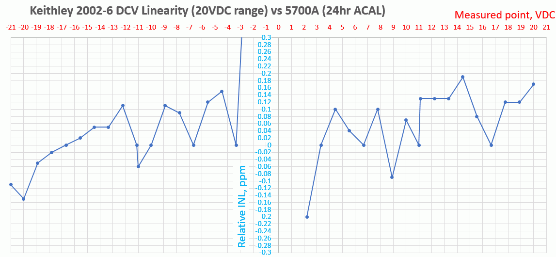
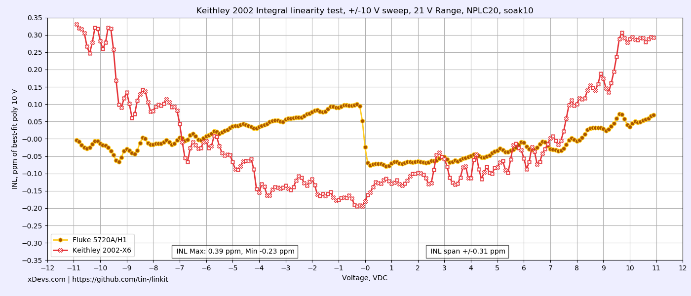
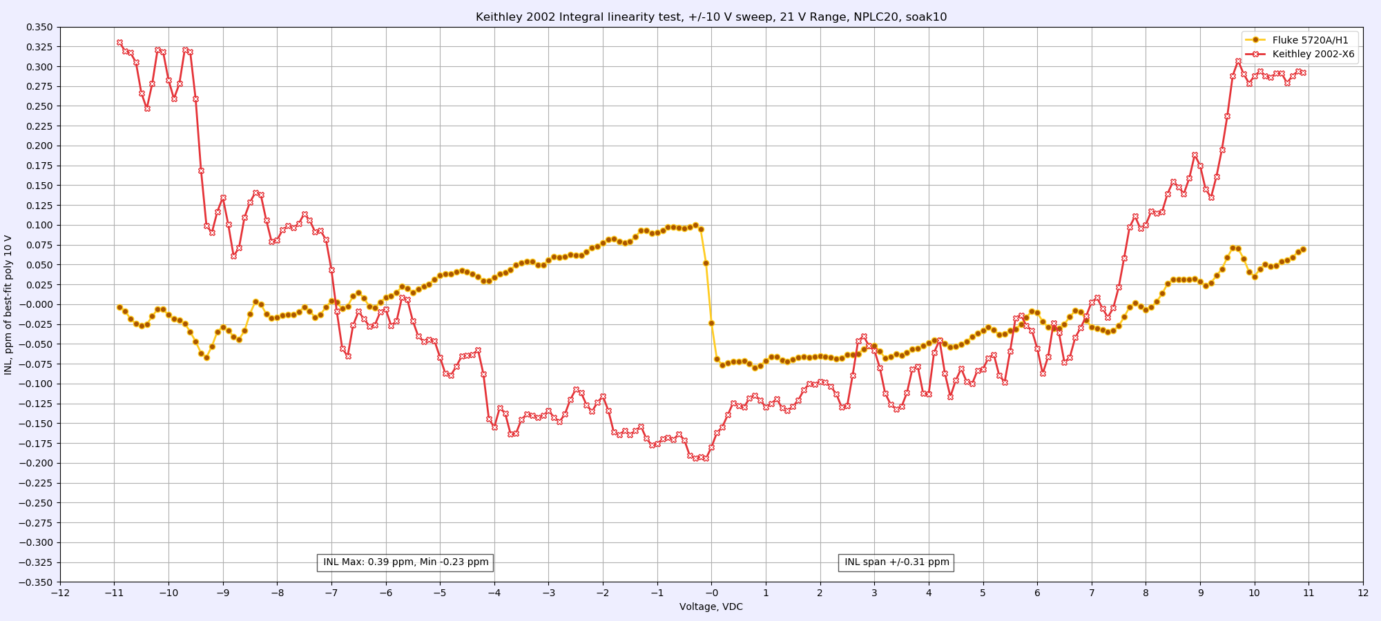
Keithley 2002-6 test on 20VDC range

On next chart another test result is displayed, plotted versus best-fit polynom from source voltage. Vertical axis span is -0.2 to +0.2 ppm/10V in 0.01 ppm step. Voltage under test is swept from -10.9 to +10.9 VDC in 0.1V increments.

Two Keysight 3458A units tested versus Fluke 5720A calibrator, using 11 VDC range

HP 3458A’s vs Fluke 5720A

One has to be careful when comparing performance specifications and read all 5pt font notes. Obviously manufacturer often may want to show “best case” result or “typical” data, leaving up to application engineer to figure out his use conditions/specifications to apply. But 3458A documentation does mention INL 0.1ppm, while Fluke let you guess from transfer specs. In my calibration verification procedures, I follow HP’s way and test against these strict levels for FAIL/PASS. I have seen that good working 3458A in shape able to deliver better than 24hour specs across whole DCV function using this worse case scenario, so for our own testing there is no benefit going the typical(?) metrology squared root uncertainty calculation.

Another thing about the above mentioned 1kV transfers. Heating/divider PCR error IS included in 3458A specification already. If you want best accuracy, you can indeed wait till readings settle out and then get better result for this range. Film Vishay resistor network for this is not too fancy, so obviously there was no goal for best performance in this range by design. From my brief testing, it takes about 15-20 minutes till 1kVDC signal settles to flat samples with sdev around 1ppm or better. And since 1kV range ACALed with 10V only, you don’t have this parasitic effect during the transfer.

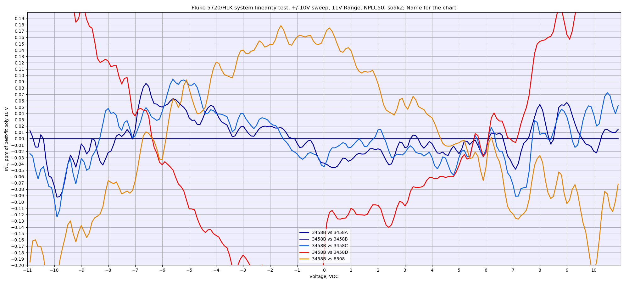
Here’s complete sweep. NPLC50, DCV10, soak time 2 second per 0.1v step, single ACAL DCV before start of sweep. Sweep is from -10.9 to +10.9VDC, take 5 readings, store median of last 3.

Graph with direct poly fit INL versus the source (Fluke 5720A “Hulk”, calibrated 2 days ago). Source considered as ideal here.

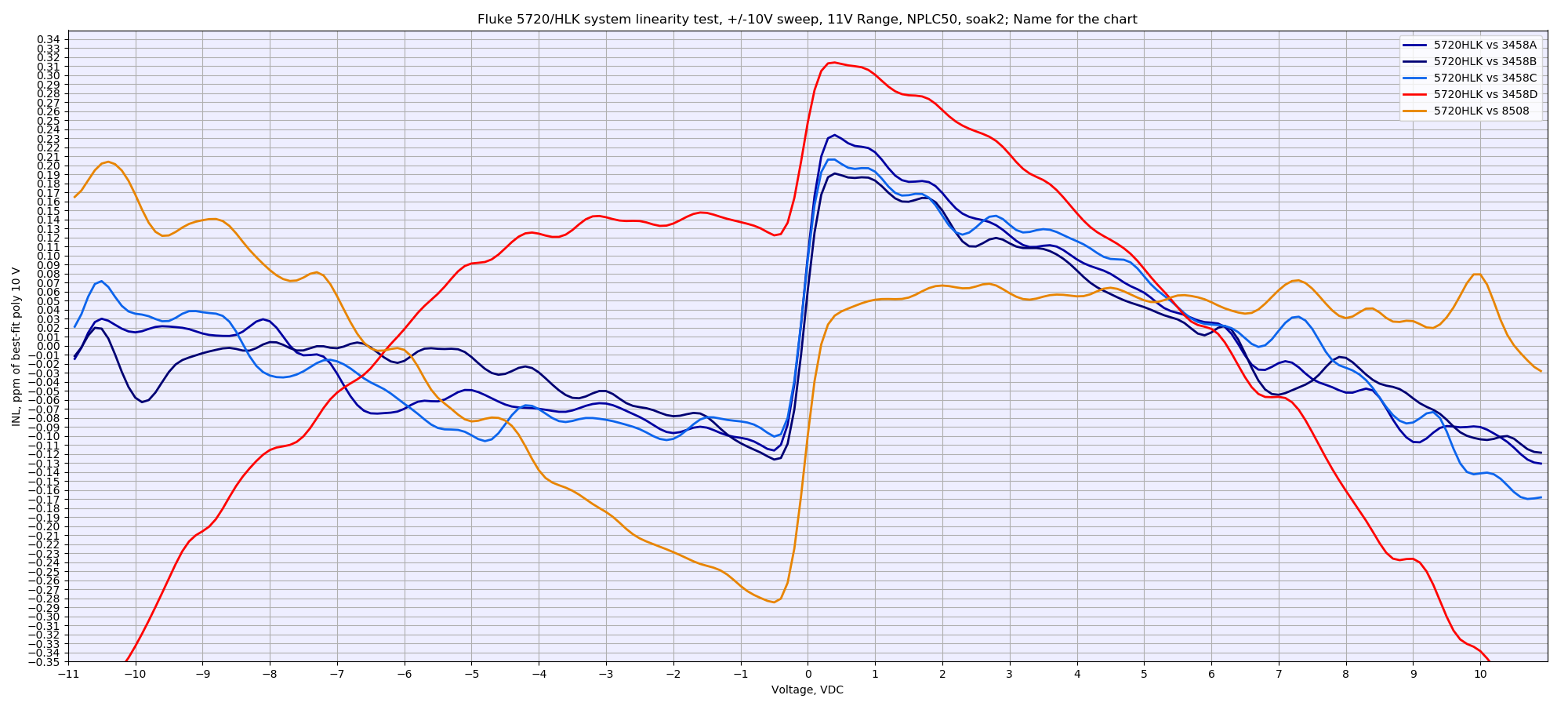
Meters A,B,C agree to each other. Can we say with good confidence that this curve dominated by calibrator’s own INL here? Questions, questions. Now question about 3458 meter D. It’s INL data is horrible, aye? Well, here the confirmation of the theory – that bad drifty A3 also gives not only drift (2ppm/day in this case) but also bad INL performance. This would be naturally expected as reference voltages are drifting wrong ways and total ratios for charge in ADC slopes would be not so good either?

I’m interested to know, as INL sweep can be faster to do then waiting for a week logging proven stable reference to find out dodgy A3 board in meter.. Fluke shows somewhat wierd data, with very good INL on positive polarity, but somewhat ugly on negative?

Now lets see on very same data, but from different angle:

Here meter “A” used as the reference, assuming it’s INL is magical 0.00 ppm. So we trade 5720A’s INL error to 3458A INL error, and can see direct difference between meter “A” and rest of the pack. Please note different vertical scale compared to previous graph, +/-0.2ppm now (previous was +/-0.35ppm).

Because three good 3458 meters agree on INL points very closely, what if we do next math acrobatics:

Reference point = ( (INL of 3458 A) + (INL of 3458 B) + (INL of 3458 C) ) divide by 3.

Now this “reference across the hospital” used as zero and each meter compared to it, showing deviation from the averaged “corrected out” 5720 INL. This idea implemented on next graph:

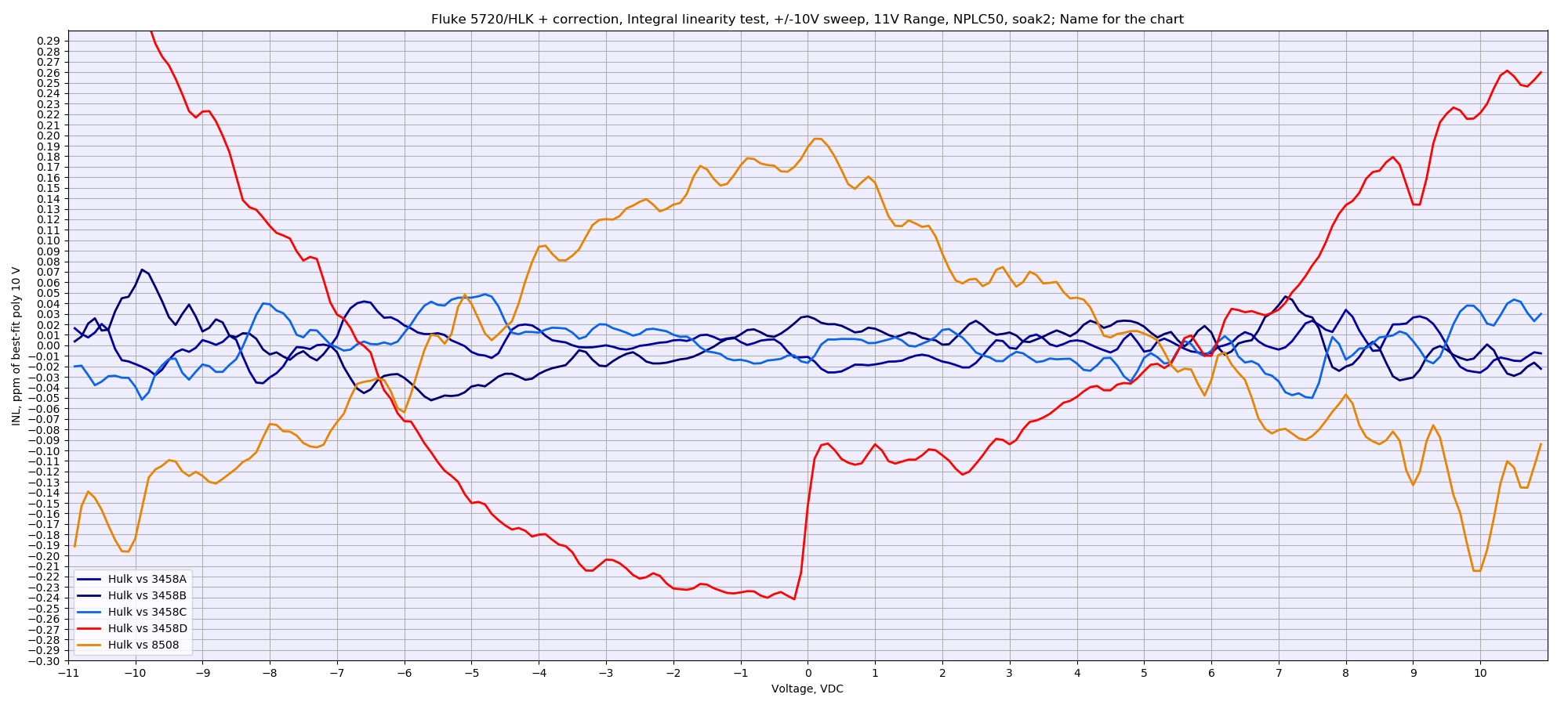
This data finally delivers long desired “typical” +0.05/-0.05 ppm across the whole sweep. If this is real or not, we will find out only next year, when my experiment extend to the next level. :-X

Perhaps same conclusion done by Jim Williams during his design for AN86 20-bit DAC, as we also see three 3458A’s on the bench. It should be clear why need to use minimum three meters, better more to better remove errors of the source itself. Please note different vertical scale compared to previous graph, +/-0.3ppm, increased to fit Fluke 8508 INL.

Also while at it, I was thinking how we can show “noise” or variance of the INL points? Previous graphs show nice and baby smooth curves, but they are not precisely true. Those datasets also hide some information from you , as each 0.1V step is actual median from 3-10 samples (depends on sweep config) so it’s not a single reading from meter. Idea was to reduce short-term noise from the meter’s ADC/REF, etc. But what if I want more real-life data, I cannot remove the inherent noise.

So instead of doing medians on step samples, I’ve ran sweep and stored every single sample into DSV file. Then same math plotting was applied with poly fit, but now twice. One is filtered out gaussian value of the step, show on graph with bright line. And peak-peak each sample data is now also plotted in opaque thick line. This gives some represenation of “peak-peak” window on each step point.

Current example, taken by another 5720A and two old 3458A’s in far far away country over remote Raspberry Pi log:

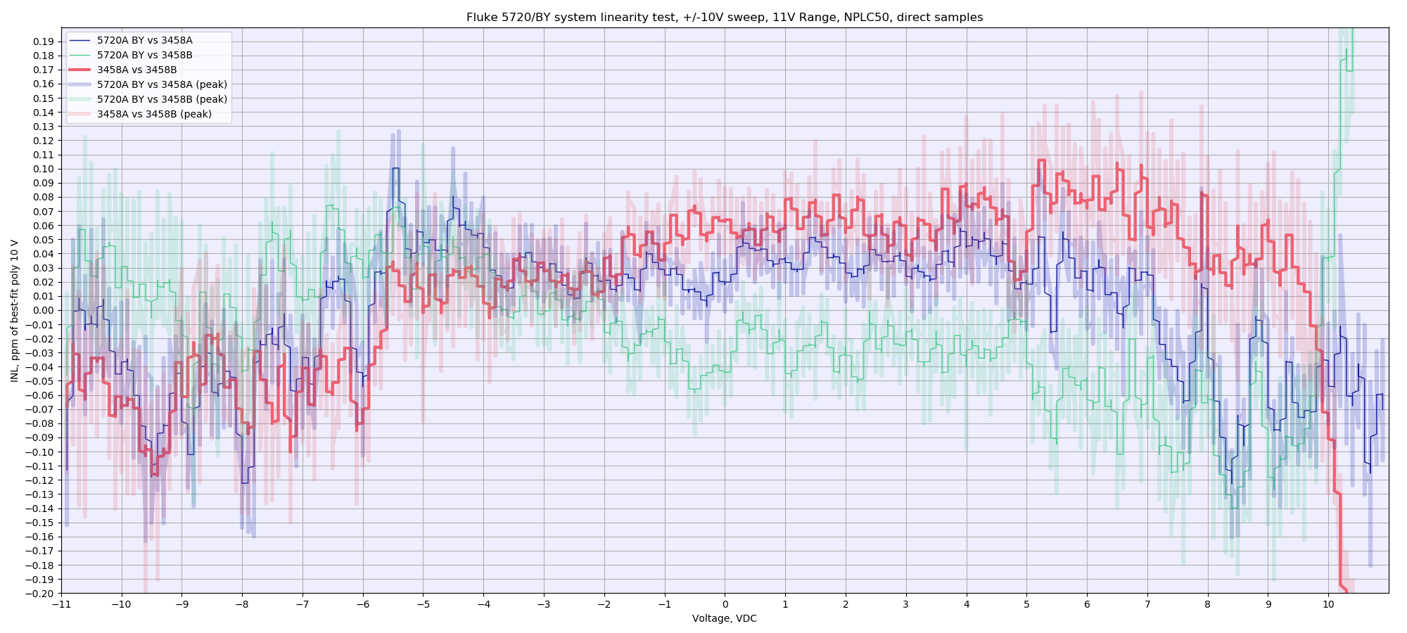
Red is differential INL between meters. And don’t ask me what happen with meter “B” after +10V…

What really amazes me – that we can even distinguish this kind of numbers at fractions of 0.1 ppm, in our crude homelab setups (even with more reasonable 5440B/4808 calibrators, no need 5720’s for this data testing). Just to think about it, own LTZ1000A reference noise that is installed in the meter produce noise around 0.2ppm all by itself, but here we looking at tiny signal deviations 5 times less than this noise! I did not really expect it.

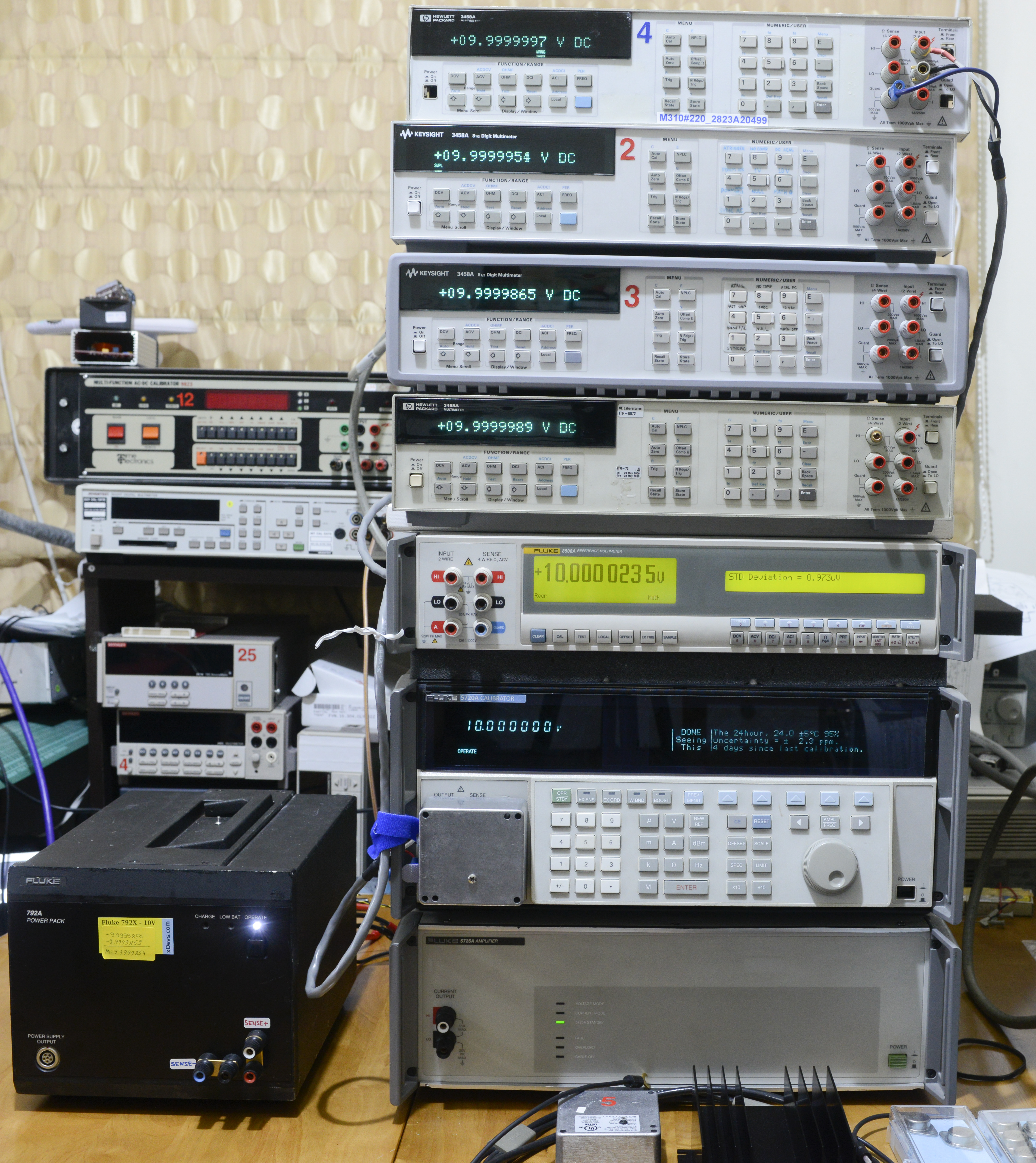
HP 3458A tandem and Keithley 2182, source = Fluke 5720A

Direct connection with Keithley low-thermal cable for nanovoltmeter, and Fluke spade lug cables for the 3458A’s. Calibrator is locked on fixed 11VDC range. Keithley 2182 running firmware A07, calibrator firmware is 1.4+ for outguard, Rev.B for inguard. HP 3458A meters configured as DCV 10, NPLC 50, NDIG 8, TRIG AUTO, MATH OFF. Keithley 2182 configured :INIT:CONT OFF;SYST:PRES;FORM:ELEM READ;ABOR;SENS:FUNC ‘VOLT:DC’;SENS:VOLT:CHAN1:RANG 10;SENS:VOLT:NPLC 5;SENS:VOLT:DIG 7. Only channel 1 measured on the Keithley unit, as input routed to same ADC path and linearity performance expected to be same between channels.

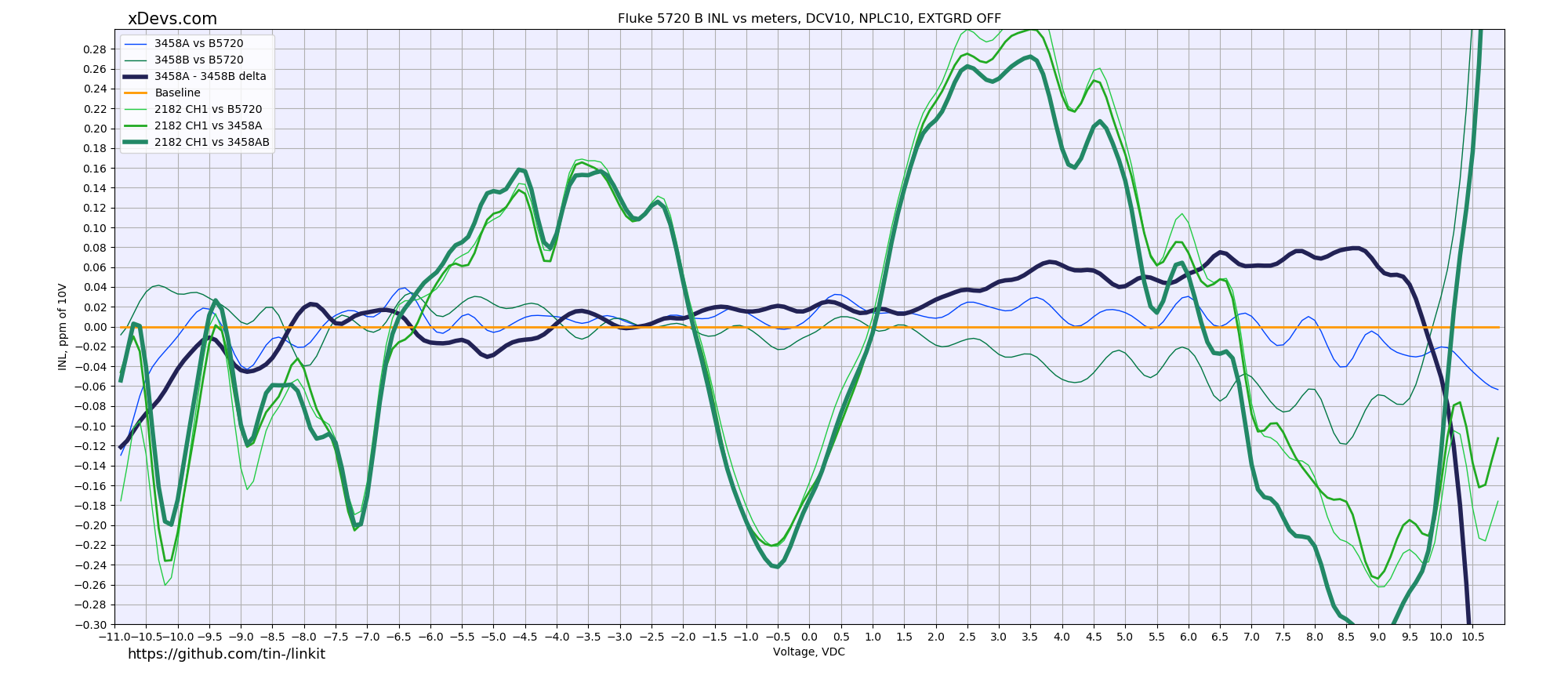
INL error plotted versus best-fit polynom from source voltage. Vertical axis span here is -0.3 to +0.3 ppm/10V in 0.02 ppm step.
Voltage under test is swept from -10.9 to +10.9 VDC in 0.1V increments.

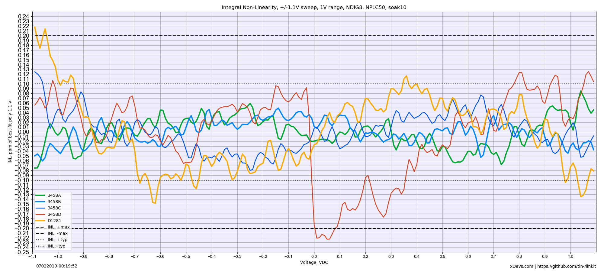
Same test sweep also repeated over -1.1 to +1.1 range, using 1V range.

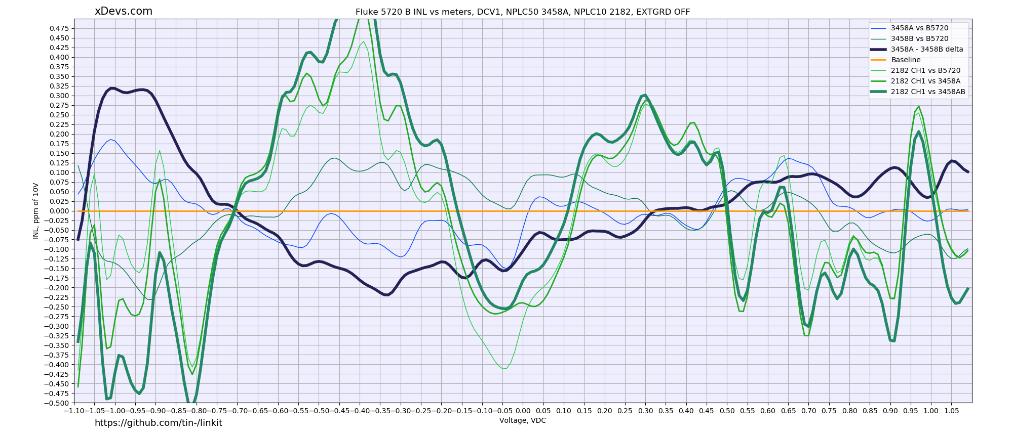
1V Vertical axis span is -0.5 to +0.5 ppm/1V in 0.025 ppm step. Voltage under test is swept from -1.09 to +1.09 VDC in 0.01V increments.

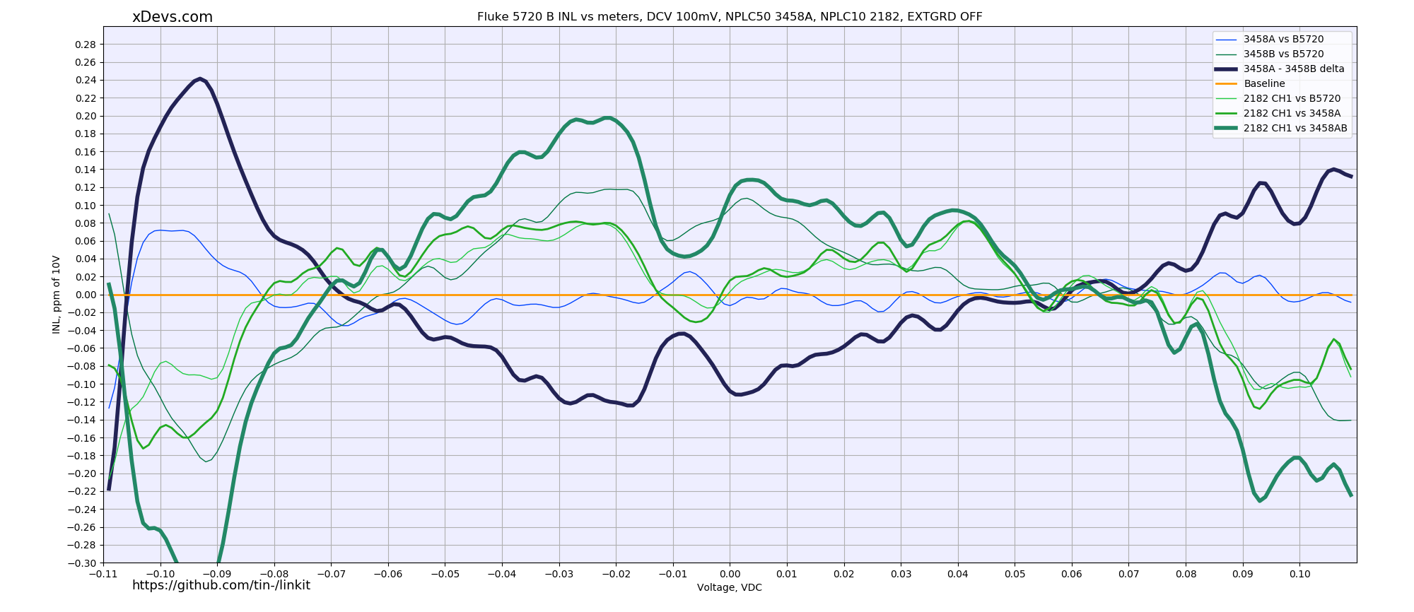
And for 100 mV range. Vertical axis span is -0.3 to +0.3 ppm/100mV in 0.02 ppm step. Voltage under test is swept from -0.109 to +0.109 VDC in 0.001V increments. For reference, 0.1 ppm of 100mV is just 10 nanovolts!

Most sensitive range 10mV. Vertical axis span is -30 to +30 ppm/10mV in 1.0 ppm step. Voltage under test is swept from -0.0109 to +0.0109 VDC in 0.0001V increments. For reference, 0.1 ppm of 10mV is just 1 nanovolt!

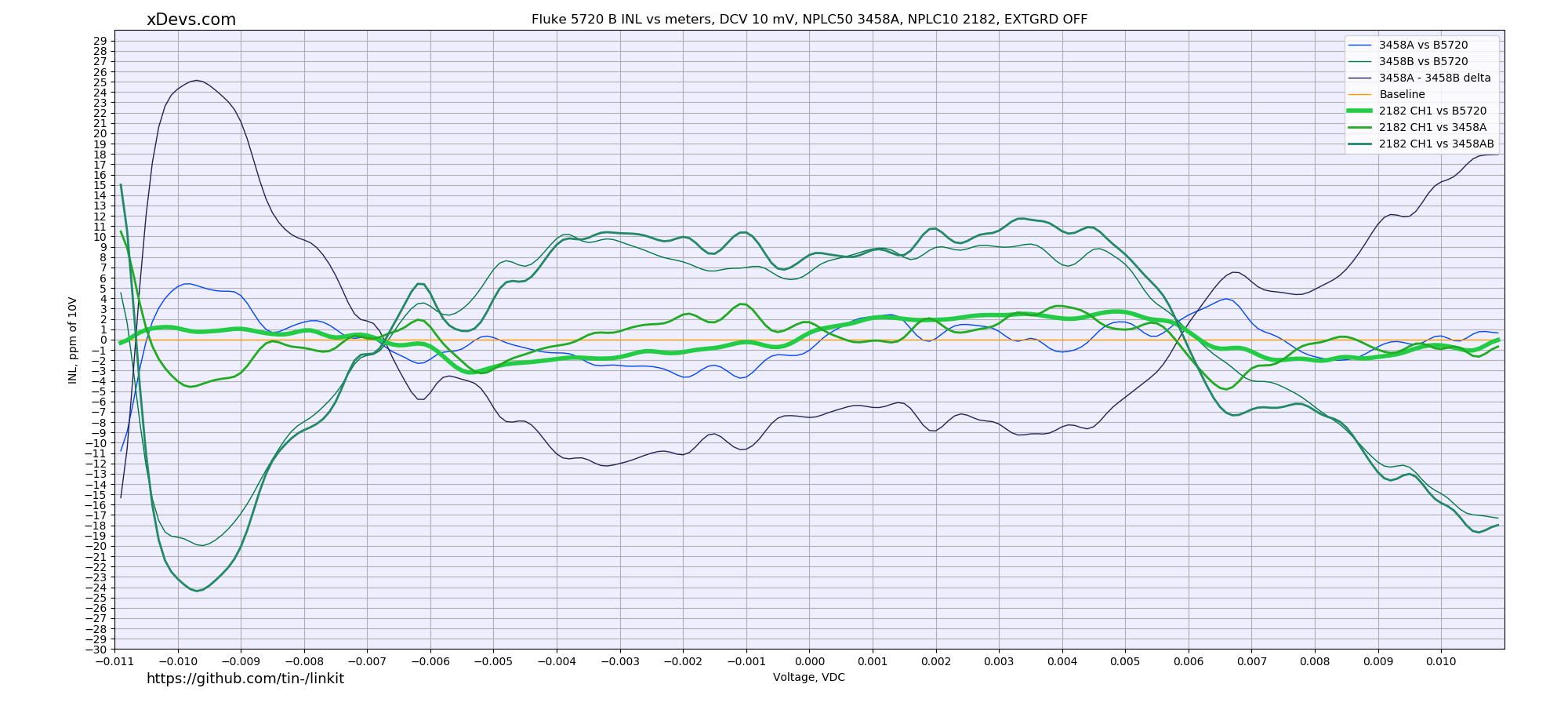
Keithley 2182 even with direct connection to MFC managed to demonstrate system INL less than ±3ppm. Keysight 3458A is at least order of magnitude worse for such low-level signal measurement.

Python app used to log data and plot graphs.

Fluke 5730A INL evaluation

Test of new Fluke 5730A calibrator, using same 3458A from test above. Calibrator locked on 11VDC range and running outguard firmware 2.04, inguard firmware Rev.D. HP 3458A meters configured as DCV 10, NPLC 50, NDIG 8, TRIG AUTO, MATH OFF.

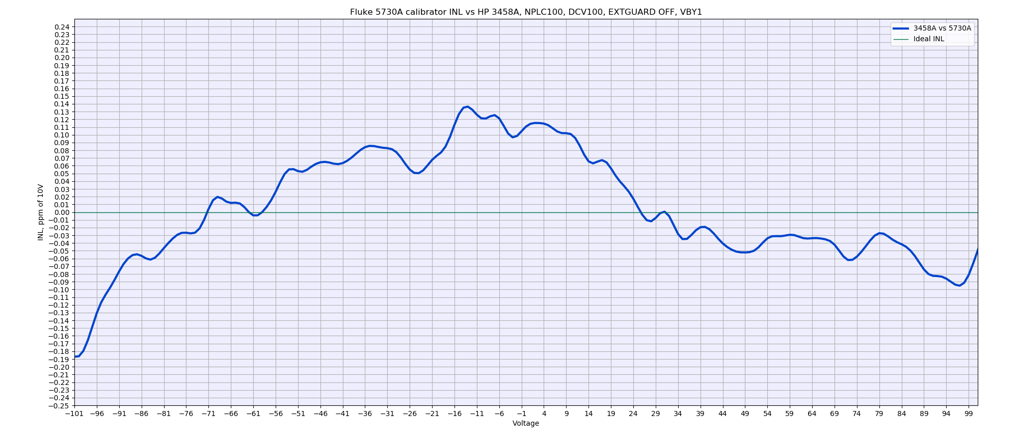
Calibrator’s 100V, HP 3458A meter configured as DCV 100V, NPLC 100. Vertical axis span is -0.25 to +0.25 ppm/100V in 0.01 ppm step. Voltage under test is swept from -100.9 to +100.9 VDC in 1V increments.

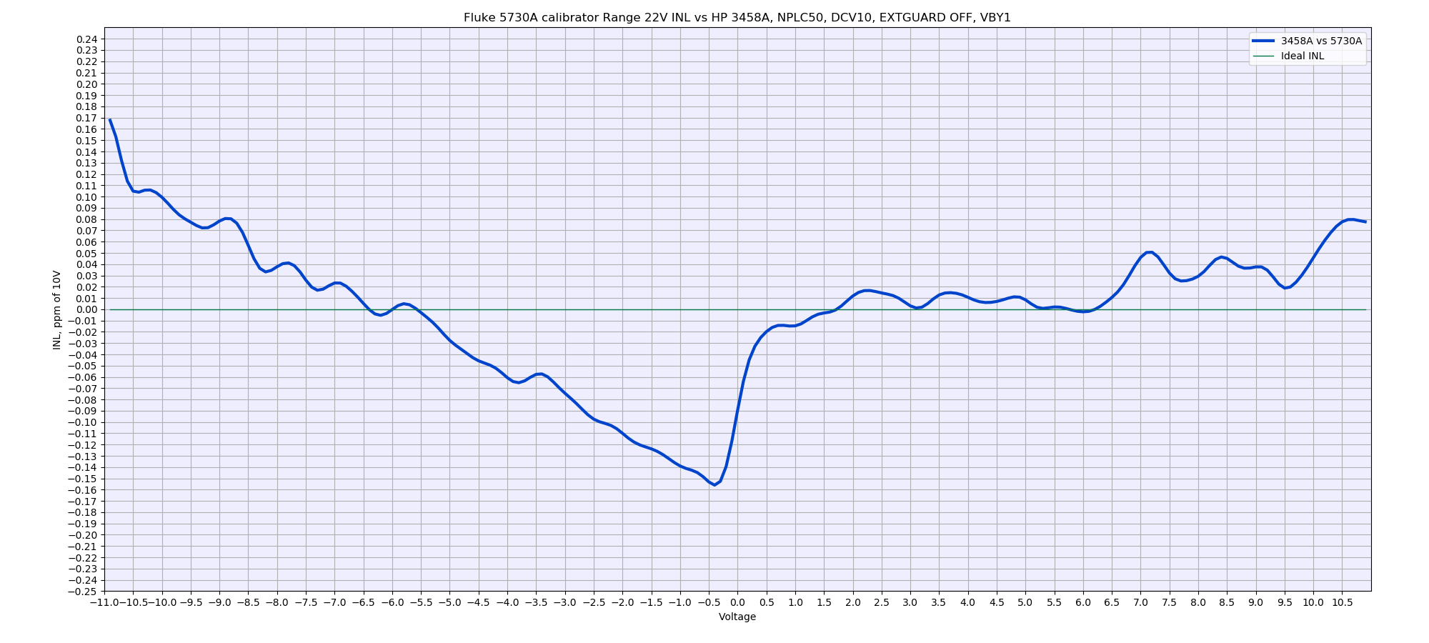
Calibrator’s 22VDC range, NPLC 50. Vertical axis span is -0.25 to +0.25 ppm/10V in 0.01 ppm step. Voltage under test is swept from -10.9 to +10.9 VDC in 1V increments.

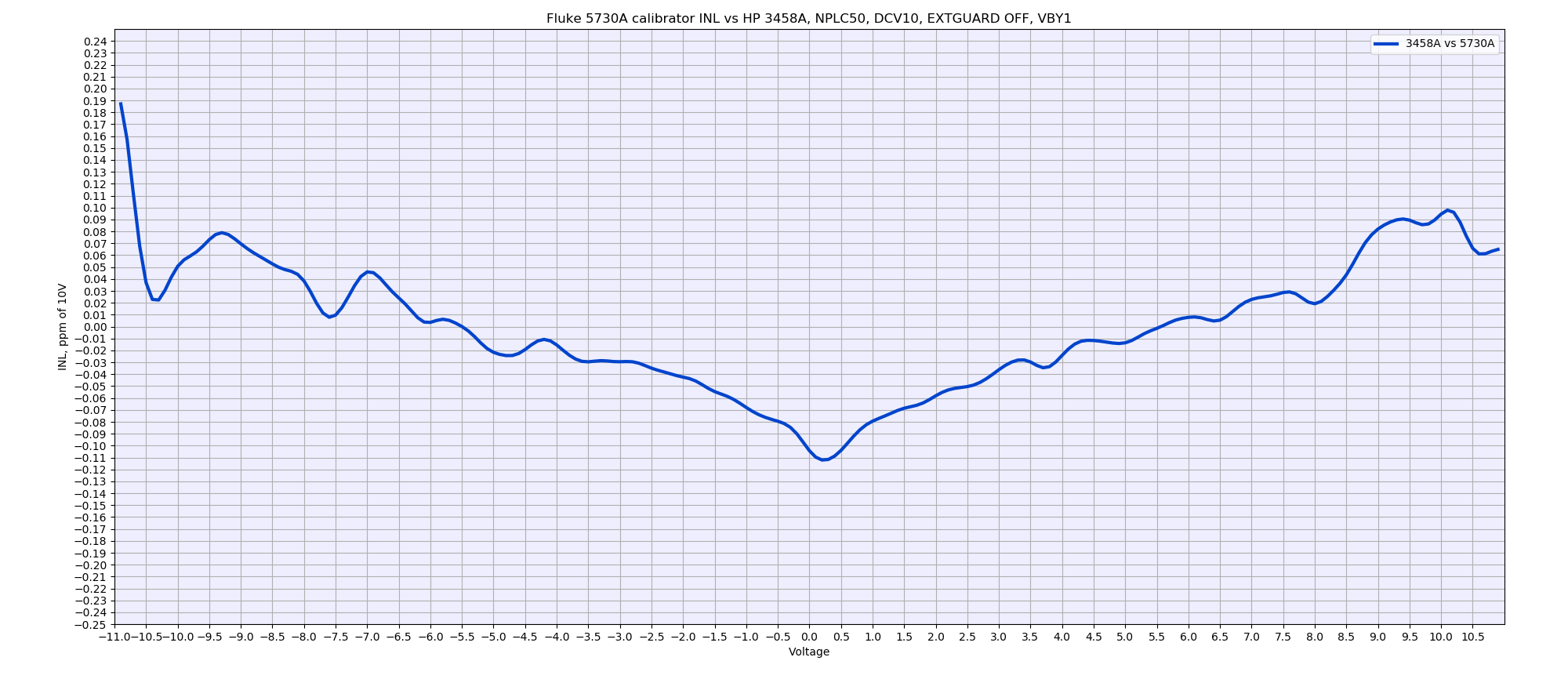
Base linearity test using 11VDC range, NPLC 50

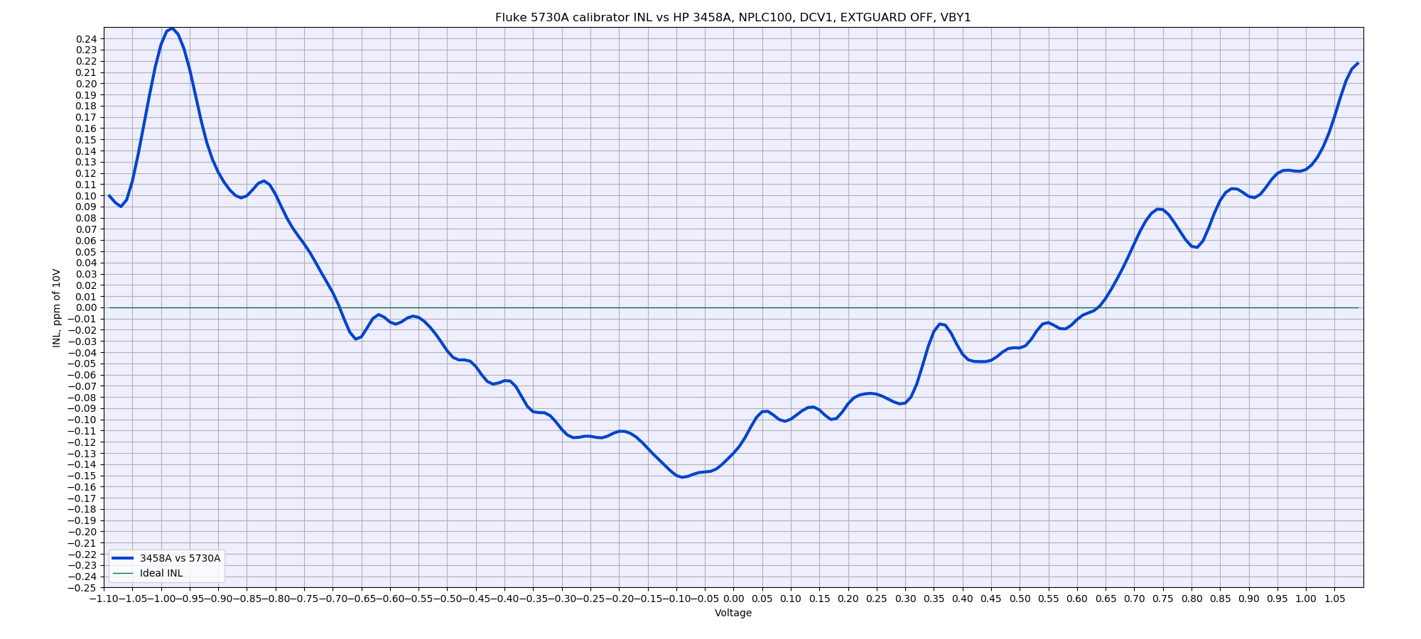
HP 3458A meter configured as DCV 1, NPLC 100.

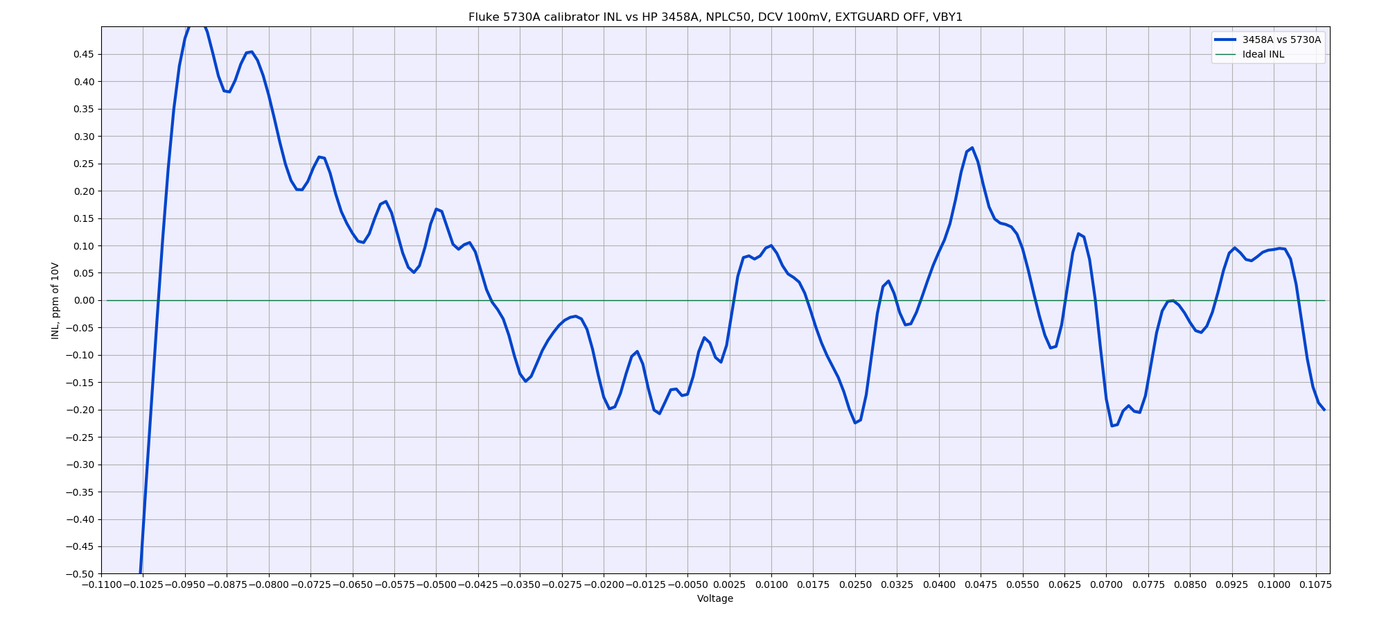
Calibrator 220mV range, HP 3458A meter configured as DCV 100 mV, NPLC 50. Vertical axis span is -0.5 to +0.5 ppm/100mV in 0.05 ppm step. Voltage under test is swept from -100.9 to +100.9 mVDC in 1mV increments.

xDevs TW Lab tests

HP 3458A tandem versus bad A3 ADC HP3458 (drift over 2ppm per hour)

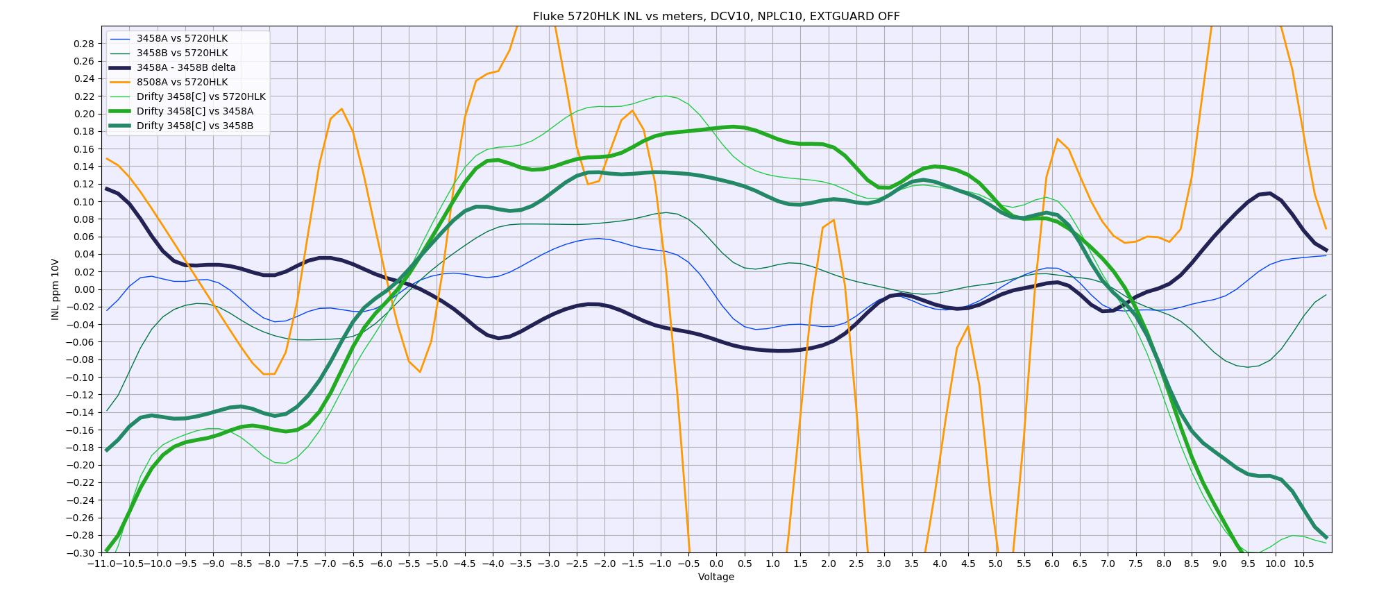
HP 3458A tandem versus Fluke 8508A and Keithley 2002⁴

Direct connection with Keithley 2002 using Fluke 5440A-7002 low-thermal cable. 3458A’s and 8508A connected with low-thermal copper spade lug cables. Calibrator Fluke 5720HLK is locked on fixed 11VDC range. Keithley 2002 running firmware A09, calibrator firmware is 1.4+ for outguard, Rev.B for inguard. HP 3458A meters configured as DCV 10, NPLC 10, NDIG 8, TRIG AUTO, MATH OFF. Keithley 2002 configured :INIT:CONT OFF;SYST:PRES;FORM:ELEM READ;ABOR;SENS:FUNC ‘VOLT:DC’;SENS:VOLT:DC:RANG 10;SENS:VOLT:DC:NPLC 20;SENS:VOLT:DIG 8. Fluke 8508A configured as RESL6,FAST_ON.

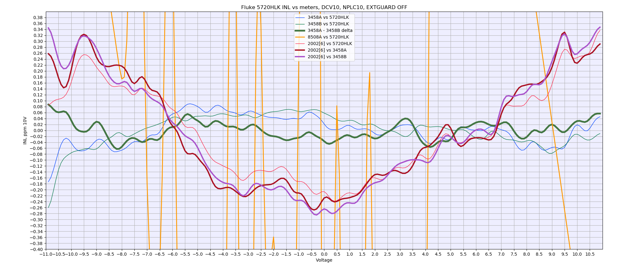
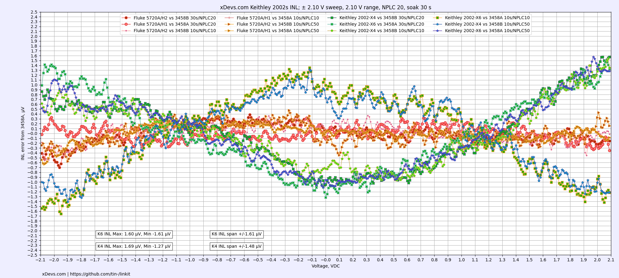
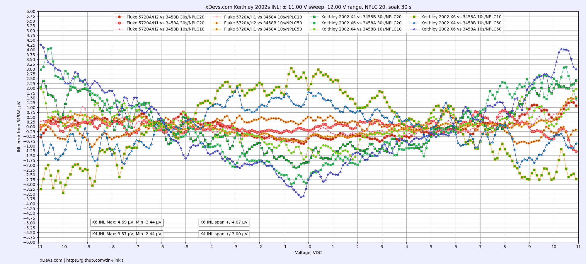
Two 2002 vs two Fluke 5720A

Operator errors and precise timing of INL sweep is ensured by automating this test with Python application. Demo code example used to perform such INL benchmark on 10V sweep is provided below for reference. It can be easily modified to test other ranges / sweep points.

Python 3 program source code to collect INL data points with K2002

This application perform configuration of source (Fluke 5720A), reference DMM (HP 3458A) and DUT Keithley 2002 DMM. After configuration is completed ACAL DCV is executed on the reference 3458A DMM and data collection of voltage sweep from -FS to +FS begins. Each data point is increased by 1% step and multiple samples are taken to reduce influence of the sampling noise. Results are recorded into semicolon-separated CSV file on the filesystem. Whole test takes few hours to complete.

Example test records DSV-file with 219 captured INL data voltage points

This datafile can be now used to plot visual X-Y chart for easy visual representation of INL performance. Python 3 again can help us here with numpy and matplotlib libraries for correlation analysis. Data between DUT DMM is reference DMM is correlated using best fit function and residual INL error is displayed relative to DUT DMM range. For easier understanding relative parts per million (ppm) scale is used.

Python 3 LinKit program to analyze and plot data

Configuration of the program, input filename, plotting parameters and chart scales are defined in separate configuration file linkit.conf. Make sure it is placed in same folder to linearity_plot.py program.

INL LinKit plotter configuration file

Finished plots are shown with simple GUI window and also saved into two images in PNG-format. Larger PNG image can be used for print or presentation, while smaller version is provided as thumbnail on web-page article like this one. Filename of the saved PNG image set is matched to input datafile name. Image files will be overwritten if they already exist in current directory.

INL LinKit plotter large PNG-image file output

INL LinKit plotter small PNG-image file output

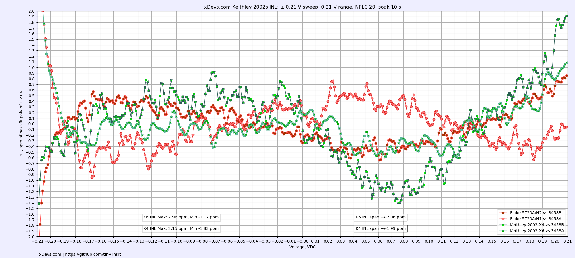
Two identical setups like shown above were used to plot two separate DUT Keithley 2002 DMM comparison.

Plotter program was modified to parse two DSV-files and generate results from each 5720A/3458/2002 system on same plot. Each 3458A used as a zero “perfect” reference.

Source code for Python 3 Dual-system INL plotter

“Configuration file for plotter program”/doc/Keithley/2002/cal2023/linkit.conf

Now the data files with samples acquired from the instruments:

DSV-file for K2002 GPIB4, 5720A/H2 and 3458B, 210 mV sweep

DSV-file for K2002 GPIB6, 5720A/H1 and 3458A, 210 mV sweep

DSV-file for K2002 GPIB4, 5720A/H2 and 3458B, 2.1 V sweep

DSV-file for K2002 GPIB6, 5720A/H1 and 3458A, 2.1 V sweep

DSV-file for K2002 GPIB4, 5720A/H2 and 3458B, 11 V sweep

DSV-file for K2002 GPIB6, 5720A/H1 and 3458A, 11 V sweep

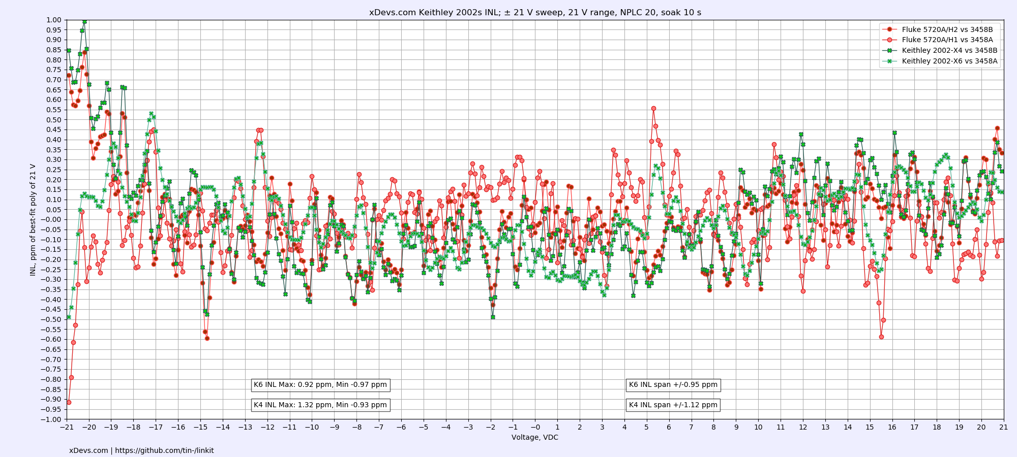
DSV-file for K2002 GPIB4, 5720A/H2 and 3458B, 21 V sweep

DSV-file for K2002 GPIB6, 5720A/H1 and 3458A, 21 V sweep

DSV-file for K2002 GPIB4, 5720A/H2 and 3458B, 110 V sweep

DSV-file for K2002 GPIB6, 5720A/H1 and 3458A, 110 V sweep

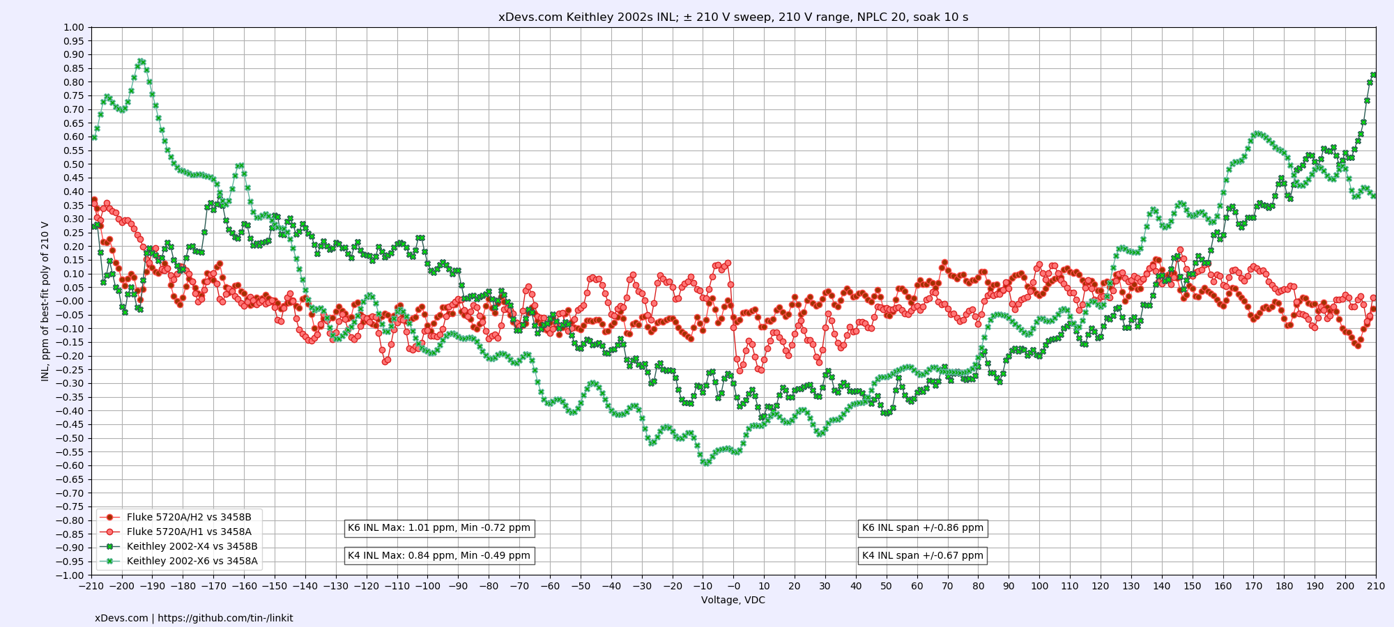
DSV-file for K2002 GPIB4, 5720A/H2 and 3458B, 210 V sweep

DSV-file for K2002 GPIB6, 5720A/H1 and 3458A, 210 V sweep

Now to results. Correlation between reference HP 3458 DMM and calibrator shown in red plots (one per system) and correlation between HP 3458A and DUT K2002 (one per system) shown in green plots.

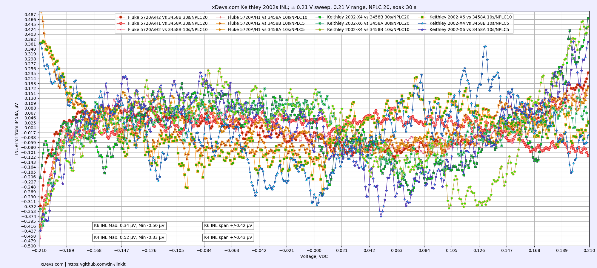
Comparison of different NPLC settings:

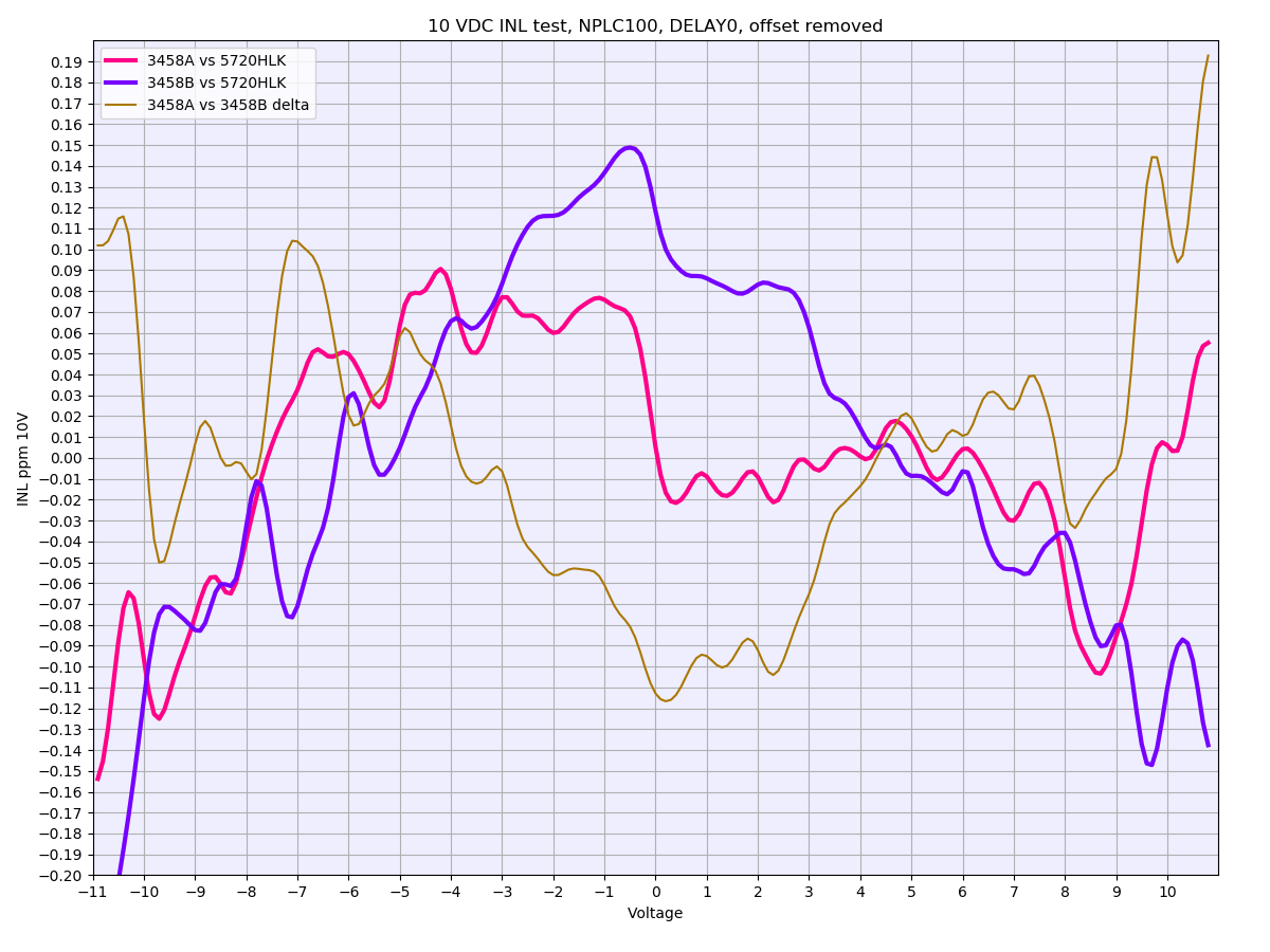
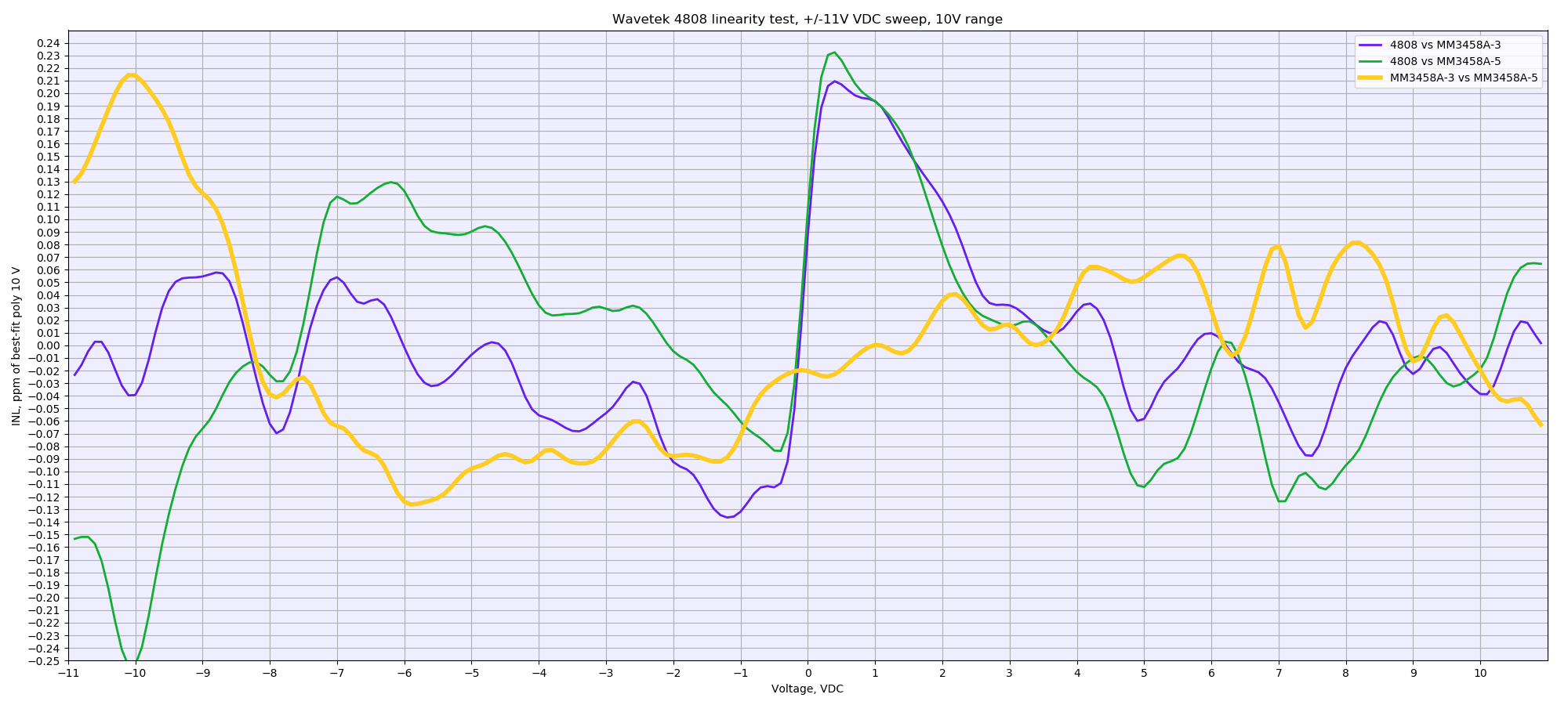
Wavetek 4808 tests with MM’s 3458A units

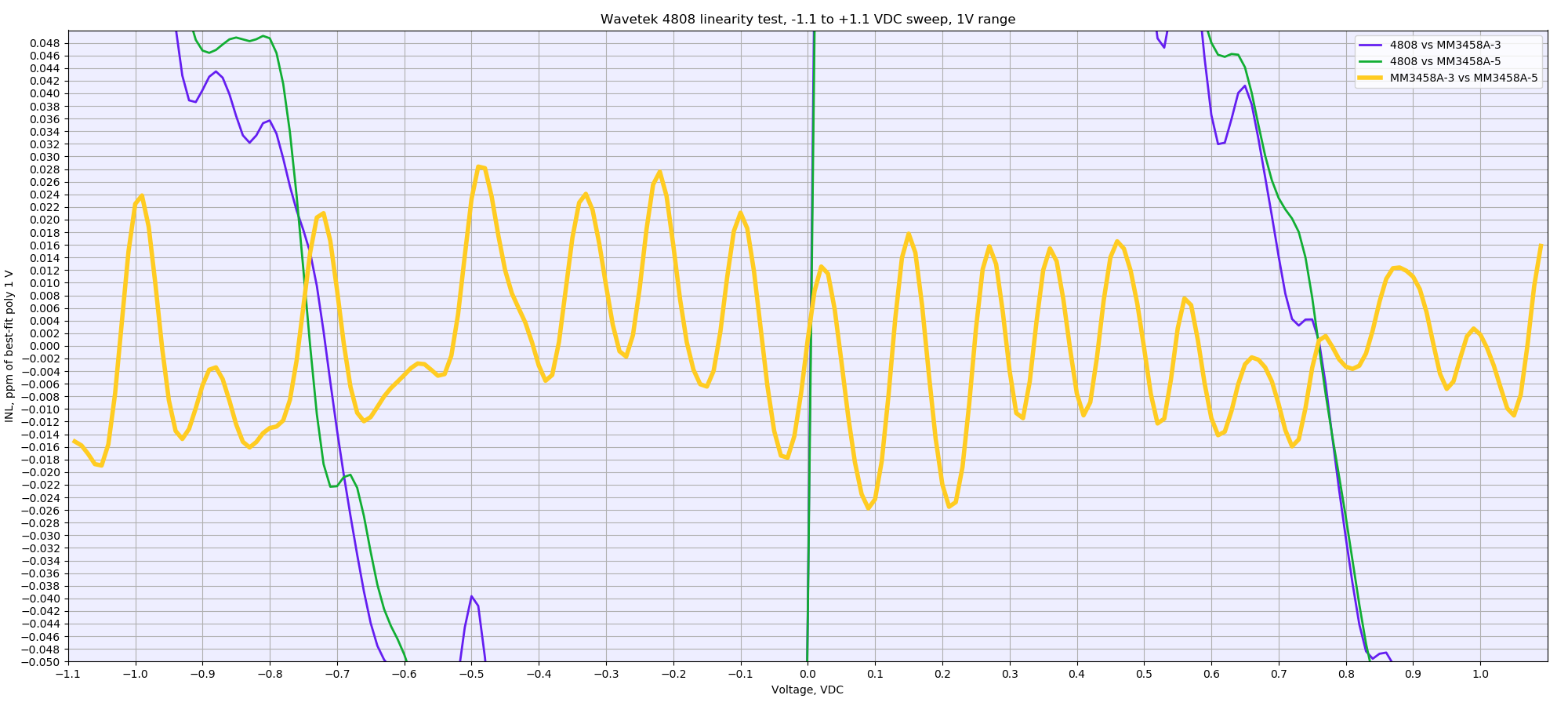
Data sampled every 1% step from -110 to 110% of the scale. Both meters configured NPLC100, DELAY0, AZERO ON and ran DCV ACAL before test start. Data might be still compromised by aircon, as it’s kinda wobbly during the sweep. Purple and green charts are direct INL of the meter vs calibrator’s programmed value. Orange line is difference between two 3458A’s used in the test. Each step have soak time 20 second after programming calibrator output to allow settling. Configuration for calibrator : S0R6F0O1=.

10V sweep. About ±0.2 ppm INL over the span. Delta INL between meters <±0.12ppm (should be at least twice better, so perhaps more tuning for settings can be done). Could be also cabling issue or thermal EMF offset, to cause the zero crossing jump. I’m not very familiar with 4808 INL performance to judge now.

1V sweep is more interesting, in respect of delta INL between meters :)

Same dataset, but zoomed in ppm INL scale to ±0.05 ppm. I’d say ±0.03ppm in full -1.1 to 1.1V sweep is impressive :-.

Now running 100mV test.

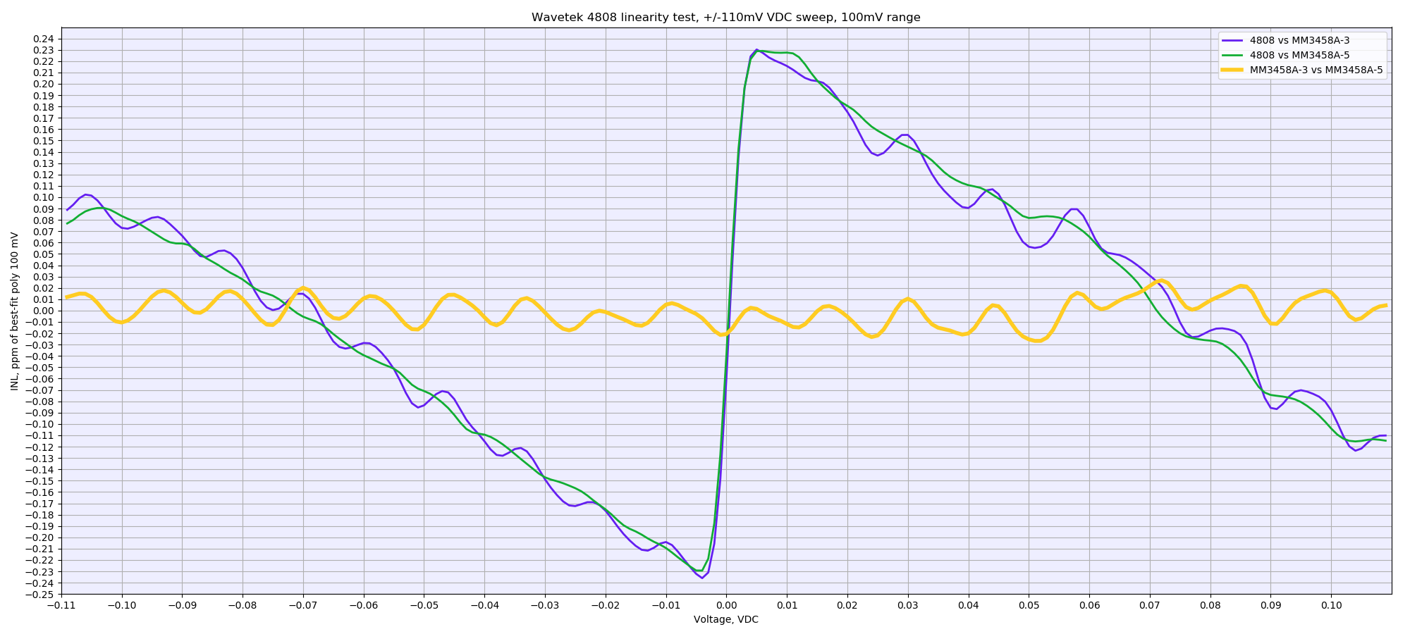
About same as 1VDC sweep, with max INL error ± 0.03 ppm. Chicken dinner winner.

Retest 10V again, with NPLC50 instead of 100 now:

And 100V INL sweep:

Negative polarity is somewhat strange. There is ~40 second delay on each 1V step, so it’s hard to tie that just on self-heating errors of the HV divider.

Few more sweeps with NPLC20 and NPLC20 with short delay (2s instead of 20sec):

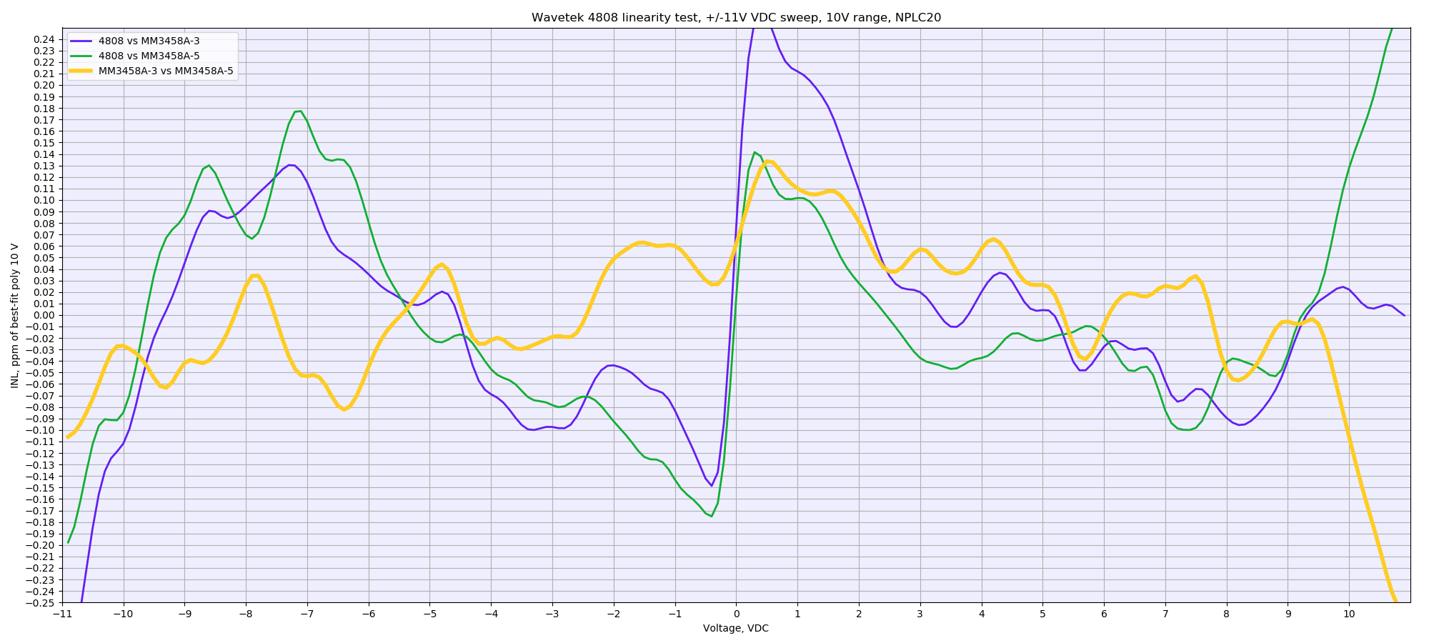
Short delay times, same NPLC20:

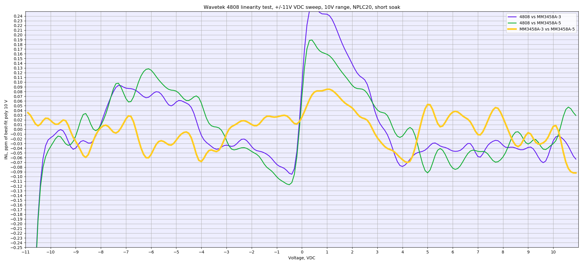
Perhaps it’s safe to assume that long NPLC100 not required to do INL test with <0.1ppm data between 3458A’s.

Datron 1281 INL sweep

Datron 1281 INL sweep was done against reference 3458A setup with 5720A calibrator. Only front input was measured in RESL8, FILT_OFF mode. Bad 3458 unit with drifty U180 was measured as well, under label “3458D”.

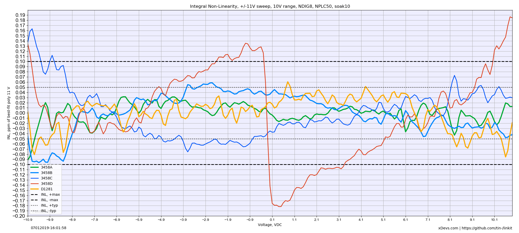
10V range is pretty nice.

1V is not too bad either.

Yet another A3 INL verification in three 3458A and 5720A/H1 setup

LinKit analyzer application perform configuration of source (Fluke 5720A), reference DMM (HP 3458A) and DUT Keithley 2002 DMM. After configuration is completed ACAL DCV is executed on the reference 3458A DMM and data collection of voltage sweep from -FS to +FS begins. Each data point is increased by 1% step and multiple samples are taken to reduce influence of the sampling noise. Results are recorded into semicolon-separated CSV file on the filesystem. Whole test takes few hours to complete.

Python application for Raspberry Pi to collect INL for three 3458A in 1 percent steps

This program ran with instruments and collected results into two CSV-files with points for further analysis.

CSV data file with 3×3458A and 5720A/H1, NPLC30, ±11V range sweep

One sweep was completed with NPLC 30 and soaking time for each point 15 seconds after new voltage is programmed in 5720A calibrator output. Second sweep was repeated with identical configuration except NPLC 50 was used on all three 3458As.

CSV data file with 3×3458A and 5720A/H1, NPLC50, ±11V range sweep

Then results were analyzed with plotter application.

Python 3 LinKit program to analyze and plot data

Configuration of the program, input filename, plotting parameters and chart scales are defined in separate configuration file linkit.conf. Make sure it is placed in same folder to linearity_plot.py program.

INL LinKit plotter configuration file

As we got dataset from three different DMMs we could play a little bit with correlation between different instruments and look at the differential INL data. This analysis outlines the benefit of having multiple 3458A for INL benchmarks instead of only relying on INL performance of the source which is always worse than good 3458A.

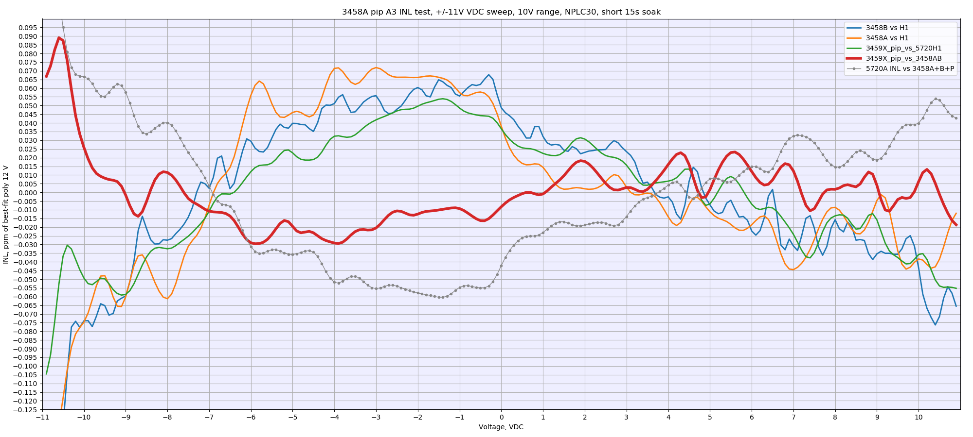
Looking at the resulted chart few more details can help with understading the legend and lines:

• Blue line “3458B vs H1” is a direct INL measurement of 3458B GPIB-1 instrument, assuming 5720A/H1 output is perfect 0 µV/V from programmed value.
• Orange line “3458A vs H1” is a direct INL measurement of 3458A GPIB-3 instrument, assuming 5720A/H1 output is perfect 0 µV/V from programmed value.
• Green “3459X_pip_vs_5720H1” is a direct INL measurement of test 3458 meter with pipelie’s A3 ADC, assuming 5720A/H1 output is perfect 0 µV/V from programmed value.

Now that we done with simple stuff and direct INL measurement from dataset, we can add few more calculated relationship INL charts. We don’t have quantum accurate JVS standard available to test INL below 0.2 µV/V directly. This means use of the 3458A DMM as automated linearity standard is the next best thing.

• Bold maroon “3459X_pip_vs_3458AB” is a calculated INL measurement of test meter with pipelie’s A3 ADC against other two 3458 INL point (3458A data + 3458B data / 2)
• Gray line with markers “5720A INL vs 3458A+B+P” is calculated INL measurement of 5720A own INL error against all three 3458A data (3458A data + 3458B data + 3459X data / 3). This is essentially a deviation of 5720A output against programmed ideal value, assuming that combined INL of the three 3458A is perfect.

And same data analysis applied to NPLC 50 datasets reveals very similar results.

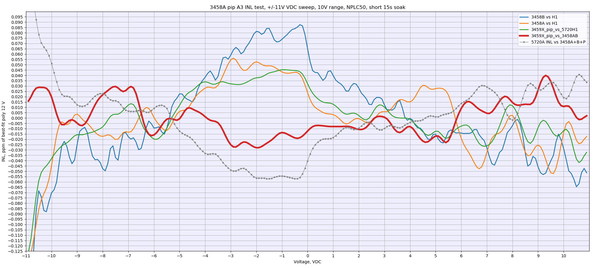
Based on these assumptions and agreement of this data with past history on our golden primary HP3458A and second HP3458A few conclusions can be made. First and most important shows the excellent performance of test A3 ADC when installed in our third test 3458X instrument. The maximum deviation window for ±10 V range sweep was inside ±0.03 µV/V and a bit worse +0.09 µV/V to -0.03 µV/V for the wider ±11 V points. This data is in a good agreement with typical good 3458A performance. This theory is also supported by nearly identical datapoints between all three independent 3458A instruments with different hardware and different ADCs if we look at direct INL datalines against “ideal” programmed value.

Second conclusion from dataset with three DMMs also confirms excellent INL performance of our specific 5720A calibrator on it’s 11 V DC range with maximum error around ±0.07 µV/V except the very extreme of negative voltage points below -10.4 V. Perhaps this extra error was due to some initial settling time as my script runs sequence of sweep voltages starting from -10.9 V and finishes it at +10.9 V.

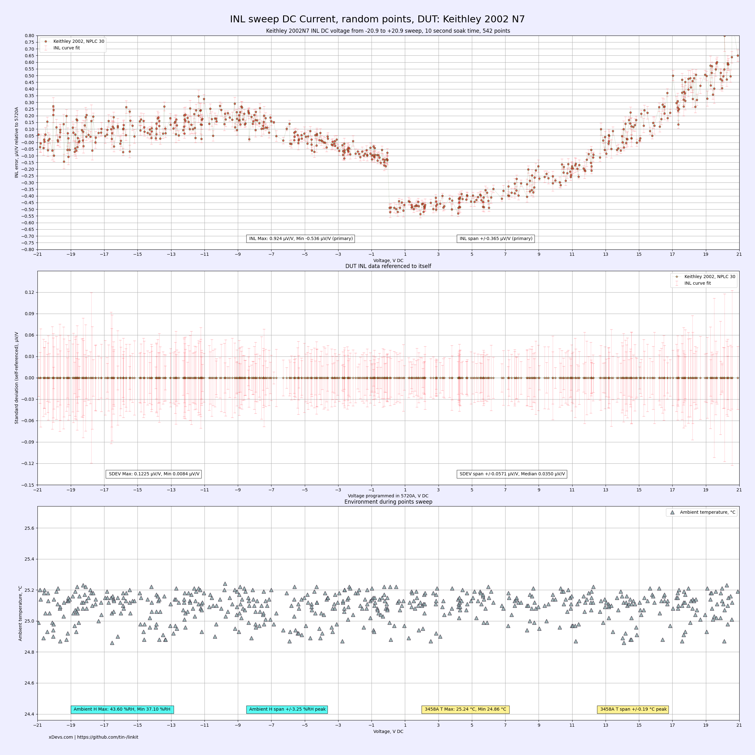
INL sweep on yet another Keithley 2002 versus Fluke 5720A/H1 or HP3458A

Often after performing adjustment and calibration on DMM we run a more detailed INL performance verification for main DC Voltage ranges. Such was also done for recently adjusted and calibrated Keithley 2002 DMM, S/N 0727052

First I’ve tested 21V sweep directly against the Fluke 5720A. This calibrator has native 22V range that can support the extended range of Model 2002.

Then I’ve added 3458A and tested limited to ±10.9 V sweep.

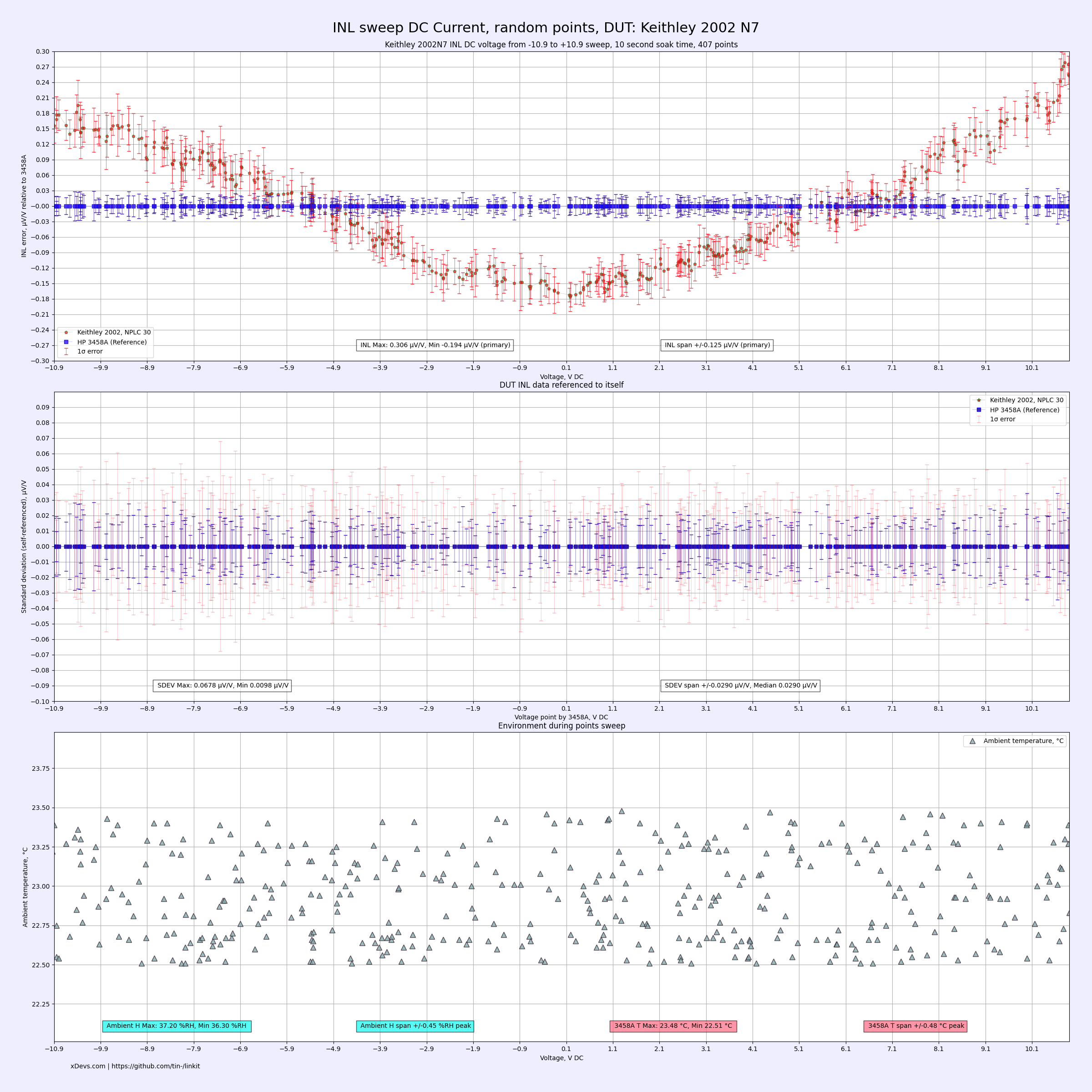
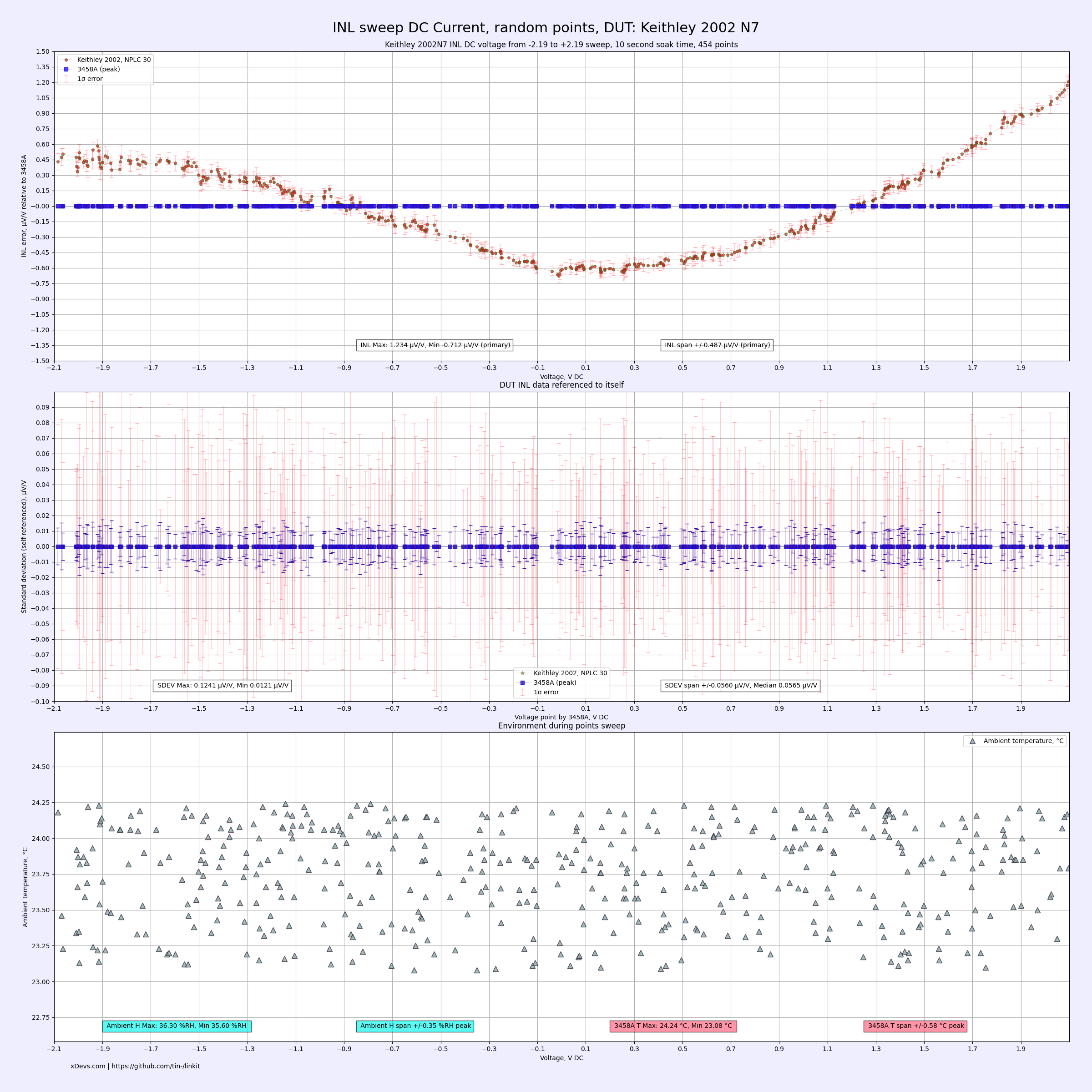
And once again with lower 2.1V range, using 2.2V range on calibrator but 12 V range on 3458A.

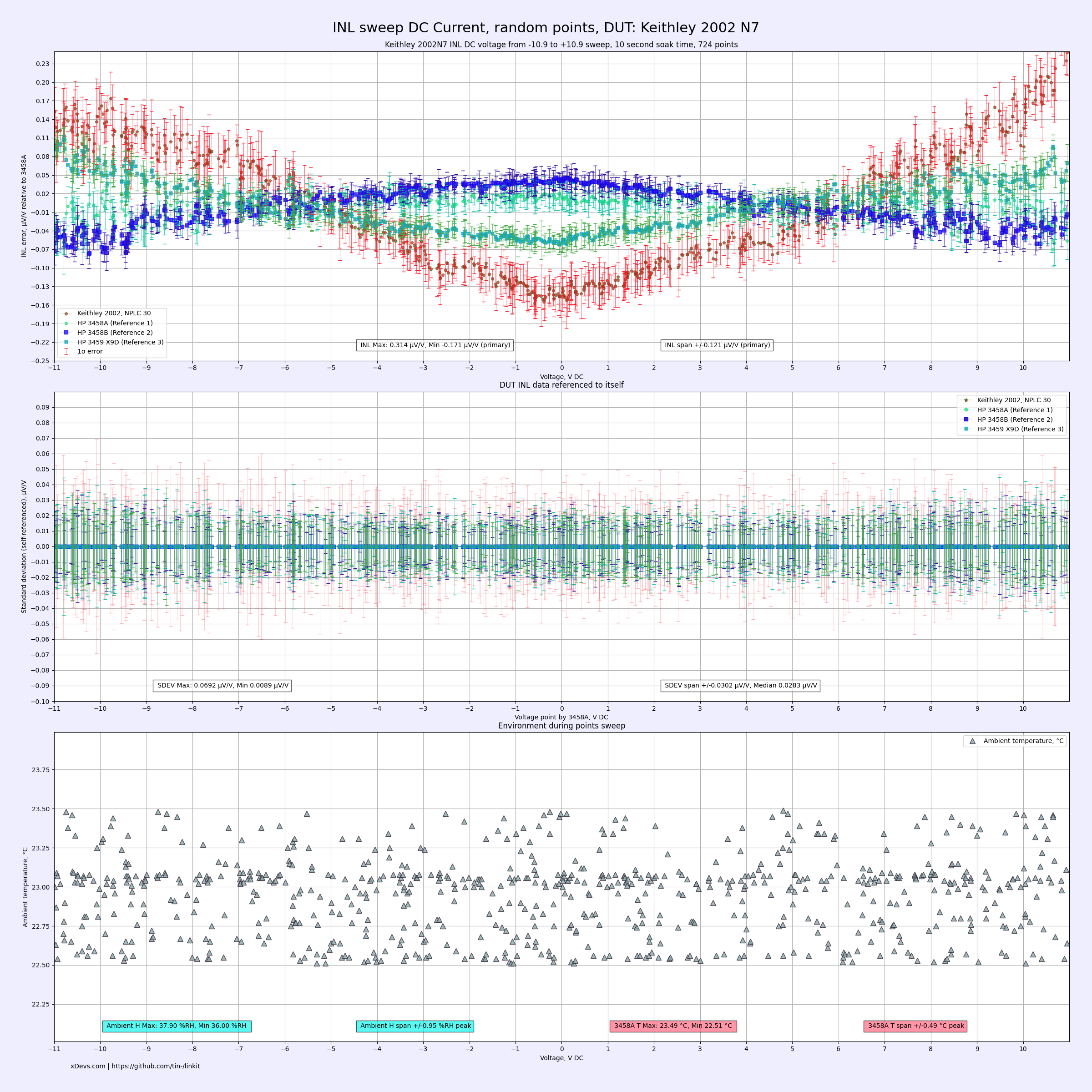
Retest with additional 3458A meters added into the group. This allowed to compare INL in respect to tandem of three 3458A instead of assuming of “reference” INL from just one meter. This test was completed with ±10.999 V sweep in random points. Data however is quite similar, meaning that measurements above were also in good agreement, even without 3458A.

All data files also available here.

Data-points DSV file for INL sweep on K2002 and one 3458A, ±10.9 V bipolar, sorted by amplitude

Data-points DSV file for INL sweep on K2002 vs 5720A direct, ±20.9 V bipolar, sorted by amplitude

Data-points DSV file for INL sweep on K2002 and one 3458A, ±2.1 V bipolar, sorted by amplitude

Data-points DSV file for INL sweep on K2002 and three 3458A, ±10.999 V bipolar, sorted by amplitude

Summary

Discussion about this article and related stuff is welcome in comment section or at our own IRC chat server: irc.xdevs.com (custom port 6010, channel: #xDevs.com).