Contents
- Intro
- Disclaimer
- Pressure, what it is, and how to measure it
- A/D signal conversion intro
- Overview on sensor design and construction
- Test setup and methodology
- Interfacing pressure sensors to Raspberry Pi using Python
- Timing and output resolution tests
- Filtering and averaging tests
- Temperature / power supply dependency test
- Calibration test
- Summary & Conclusion
Intro
Unlike digital electronics and Internet space real world is based on many complex analogue-type universe laws. Everything interacting, changing and constantly evolving, from microscopic atoms to galaxy-sized events in space. Today’s advancement in science and technology brought us powerful computers, mighty measurement tools and many comprehensive methods to learn. This all to help us analyze different aspects of world around us, study and better understand underlying rules. And often vital interface, crucial link between abstract math and theory with the actual matter is some set of sensors. Engineers and scientists have sensors and tools to detect electric charge and flow, air or liquid parameters, temperature, light intensity, objects mass and time, and much more. Field of science, that ensures accuracy of all these measurement sensors is called metrology.
Regular readers may find number of articles and experiments around common electrical values, such as voltage or resistance presented in previous xDevs.com publications. Many of them focus on quantities like voltage, current, temperature and time. However, world of physics does not end here, and to expand a bit further, today will talk about pressure.
Disclaimer
Redistribution and use of this article or any images or files referenced in it, in source and binary forms, with or without modification, are permitted provided that the following conditions are met:
- Redistributions of article must retain the above copyright notice, this list of conditions, link to this page (https://xdevs.com/article/pressure/) and the following disclaimer.
- Redistributions of files in binary form must reproduce the above copyright notice, this list of conditions, link to this page (https://xdevs.com/article/pressure/), and the following disclaimer in the documentation and/or other materials provided with the distribution, for example Readme file.
All information posted here is hosted just for education purposes and provided AS IS. In no event shall the author, xDevs.com site, or any other 3rd party be liable for any special, direct, indirect, or consequential damages or any damages whatsoever resulting from loss of use, data or profits, whether in an action of contract, negligence or other tortuous action, arising out of or in connection with the use or performance of information published here.
If you willing to contribute or have interesting documentation to share regarding pressure measurements or metrology and electronics in general, you can do so by following these simple instructions.
Pressure, what it is, and how to measure it
Common definition for pressure is force per unit area that a media volume exerts on its surroundings. As result, pressure P is a function of force F and area A.
P = F/A
The SI unit for pressure is the Pascal, but other common units of pressure also include pounds per square inch (psi), atmosphere (atm), bar, inches of water (inH2O), inches of mercury (inHg), and millimeters of mercury (mmHg) and few others. 1 Pascal is equal to pressure exerted by one newton of force, perpendicularly upon one square meter area.
1 Pa = 1 N/m2
A pressure measurement can be static or dynamic. Static pressure measurement apply for zero motion of the objects (e.g. pressure of still water to the bottle walls), while dynamic pressure measurement shows amount of force produced in moving systems (e.g. water flow in the pipe). Depending on type of pressure measurement methods and sensors can vary, to better fit specific task requirements.
Pressure is exactly the force that makes hot teapot whistle. When water boils into steam, internal teapot’s volume pressure push harder on teapot walls. As there is only one tiny teapot connection with lower pressure space, nose exit, most of excessive steam pressure escapes this way creating the air flow and high-pitch sound we all can hear. When teapot cold, there is no excessive pressure, and no sound. For same reason if teapot left open, no whistle will be possible, as pressure cannot build without cap sealed.
Device to transform pressure level into electrical signal, such as voltage or current change is called pressure sensor, or pressure transducer. Modern pressure sensors have sensing element that changes its property with pressure change. This element can act as variable resistance or capacitance to produce electric current or field change with pressure application. Change of electric property can be then measured, and it will tell us what is the applied pressure to sensor. If main interest is dynamic pressure, such sensor output need to have fixed value offset removed, and provide only small change to detect small pressure changes.
Common and well-known method and circuit to measure these small resistance changes accurately is by using Wheatstone bridge. Invented in Samuel Hunter Christie in 1833, the bridge circuit was later studied by another scientist, Charles Wheatstone. Wheatstone made circuit widely known and public, and this bridge arrangement was called after his name, as result.
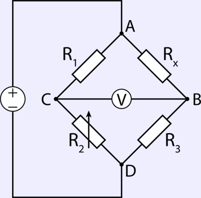
Image 1: Wheatstone resistor bridge circuit
The principle of the circuit is that if three resistances R1, R2, R3 are known, and the current in the cross branch C-B is nulled out to zero, and the fourth unknown resistance can be calculated. The measurement can be made very accurately since zero current detection can have very good accuracy.
Bridge null voltage VZ, measured between nodes CB can be calculated as:
VZ = VIN * [ RX / (R3 + RX) – R2 / ( R1 + R2 ) ],
Where VIN is excitation voltage supplied at bridge nodes A and D, and RX is unknown resistance. Here is handy real-time calculator for RX from measured VZ to get better idea, working by this very same formula. Just enter your known resistance values, and browser will calculate unknown resistance.
Resistance calculated: Ω
If special resistors that change their value under pressure are used, such bridge circuit can be used to convert physical pressure force into electrical signal. MEMS piezoelectric pressure sensor implements exactly such resistive elements, that change resistance value from applied mechanical stress. Stress to sensor introduced from pressure differential on a thin silicon membrane. Cavity under membrane can be hermetically sealed (for absolute pressure measurement) or have other pressure as reference (atmosphere for gauge sensors, second pressure port for differential measurement). Most of pressure sensors use four or more piezo-resistive elements, fabricated on the same silicon die.
As result of input pressure difference from the internal cavity pressure, the very thin silicon die membrane will get slight deformation, resulting change the resistance of sensor elements. Larger pressure stress deform element more, also changing output in predictable way. Elements typically connected in a Wheatstone bridge configuration with resistors R1 and R4 showing increased resistance with input pressure increment and resistors R2 and R3 showing resistance decrement. This provide doubled sensitivity of the sensor die to the pressure change, making measurement easier. Differential pressure sensors work same way, but using second port to open cavity to measure pressure difference between the ports. Such sensors commonly used for flow measurement, be it airflow or liquid flow. Differential pressure sensor act as pressure comparator.
Desired pressure range of the sensor is realized by variation in membrane rigidity or physical thickness/area. Sensors for higher pressure would have less stress transferred to bridge resistors, resulting lower output signal sensitivity.
A/D signal conversion intro
All this sounds great and wonderful, but how to actually design a system that converts electrical signal from sensor bridge silicon die into digital data-stream, which can be further processed, stored or displayed in user application?
Conversion of such analog voltage signal to a digital code is required. Core component for this interface between analog physical world and digital information domain is analog to digital convertor or ADC. Opposite conversion of digital code into analog signal also possible, by the DAC or digital to analog converter*, which for purpose of this article is omitted.
ADC converts input analog signal, such as voltage into a digital code determined in relation to second known signal, the reference voltage. As result sole purpose of ADC is to work as a comparator of unknown signal to known reference, with result provided in digital code. Very same idea as operation of weighing balance, to obtain ratio between two quantities, one of which is known.
Also due discrete nature of digital code, all ADCs apply quantization to input signal to obtain finite number of digital codes. Because analog signal has infinite amount of steps, it would need infinite size digital code to represent 100% of the signal. As result limiting input scale to some predetermined levels, and splitting it to small steps is required to represent input signal with close approximation. Common definition for minimum digital code step size for specific ADC is Resolution, and it is represented in bits. Ideal 1-bit ADC will generate “1” when input analog signal larger than 50% of the range, and “0” if less. 8-bit ADC have 28 = 256 steps, thus able to determine 100% / 256 = 0.390625% change of the range. If we make our range limits between 0.0V and 10.0V, then such ADC can resolve input analog signals with 39.0625 mVDC per 1 bit of digital code output.
Increased resolution reduces this minimal step size. In same example of 10.0V range ADC, 16-bit solution will provide 10.0V / 216 = 10.0V / 65536 = 152.588 µV/bit.
Simplest ADC system without any additional amplifiers or attenuators have its input range equal to known reference voltage signal. Many modern ADCs have also integrated amplifiers and front end circuits to allow multiple ranges from single known reference voltage. More details on this are covered in chapter below.
Keywords and terms, commonly used in A/D and D/A conversion applications
Bandwidth – difference between the upper and lower signal or process frequency. It is essentially a whole set of frequencies, which can carry valuable signal information of interest. Bandwidth represented in Hertz (Hz). For example, A/D system with bandwidth 0-10 kHz able to measure any signals between DC and 10 kHz. There are different challenges present in designing very accurate slow DC level converters, or high-bandwidth fast converters.
Accuracy – difference between the actual digital output and expected digital output for a known analog input signal. ADC accuracy shows how many bits from total resolution carry useful and true information about the input signal. Two ADCs with equal resolution can have very different accuracy specifications.
Calibration – measurement of ADC/system error against known accurate input signal, to determine accuracy. Calibration data can be used to perform further processing ADC’s output data to compensate for measurement errors and improve total system accuracy.
Compensation – correction process of ADC errors, based on calibration results and design constrains knowledge. Compensation can be done in digital domain (math correction of raw converted samples) or analog domain (special circuit provide error signal to adjust front-end parameters). Typical examples of compensation are using temperature sensor for thermal gain/offset errors correction, or using sensor current value to account for self-heating effects.
Standard deviation – span size of data samples variation present in the dataset. Typically, variation combines noise of the measurement/conversion system, non-linearity and other offset/gain errors. Smaller standard deviation allows to obtain better uncertainty from the dataset and higher confidence in accuracy.
Noise – voltage or current fluctuations on the signal, which can be picked up from surrounding components/environment (such as switching signal noise, RF/EMI radiation, charge pickup) or generated internally by component physical effects (such as thermal noise, present in every electronic device, even passive resistors). Noise limits the useful sensitivity of the design, essentially limiting possible conversion resolution.
Transfer function – function of relationship between input signal and output digital code. Ideal transfer function have zero INL/DNL error, no offset or gain errors. On graphical representation it looks like straight line from 0V (all bits are zero) to full scale voltage (all bits are ones).
Linearity – deviation of ideal to actual converter transfer function. Can have differential (DNL) type, which shows deviation between near code bits or integral (INL) which shows total maximum overall deviation. This deviation is very difficult to remove, as it would need accurate measurement of input signal and related digital code on all possible ADC points. INL/DNL are often used as key merit of total ADC’s conversion accuracy for any possible input signals.
Reference voltage, VREF – known voltage signal, to which input signal will be compared, or referenced. Can be either DC or AC, depending on application purposes. Using same reference voltage to feed resistance bridge allows true ratiometric measurements, reducing importance of reference voltage stability. For absolute measurements stable reference is a key component of the converter, as reference performance (noise, stability) defines meaningful resolution. Some of these aspecs were covered in better detail here, during design of ultra-stable solid-state voltage reference module.
LSB size – minimal voltage step size for each code, equal to Reference voltage / 2N.
Important note on resolution numbers
Resolution of the ADC often confused and mistaken with accuracy, but actually these two parameters are almost unrelated. Higher resolution does not provide better accuracy, it only provides smaller digital step size. Together with input signal range resolution provide sensitivity of the ADC.
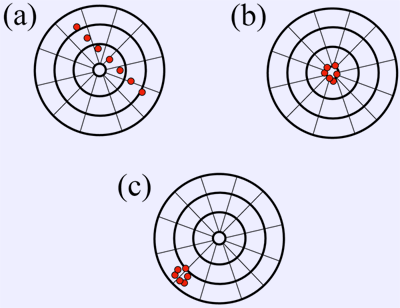
Image 2. Accuracy versus Resolution representation
Case (a) represents low resolution and low accuracy, with samples all over the place. We cannot clearly see what is true signal value. Improvement on both resolution and accuracy will get sample distribution like on case (b). This is high resolution with high accuracy. Now if we still use high resolution, but system accuracy is low, results will be case ©. That’s why calibration often more important than resolution for high-precision equipment, as even if we have high precision, it does not provide good accuracy as well.
There are many cases, when 24-bit ADC provide worse accuracy than better 16-bit device. So resolution provides theoretical sensitivity level, in terms of smallest digital code difference, while accuracy is derived from complex mix of many actual ADC design parameters, such as front end stability, temperature coefficients of amplifiers/voltage references, calibration and compensation correction and noise isolation from other components of the system.
As example, using 0-10 V range 8-bit and 16-bit theoretical ADCs, let’s convert 5.000 V analog signal into digital code, but this time with one extra variable. In case A voltage reference (known voltage against which ADC compare input signal) is precisely 10.0000 V, while in second case B there is 100 mV error in voltage reference, so true reference voltage is 10.1000 V.
| 8-bit “A” ADC | 8-bit “B” ADC | 16-bit “A” ADC | 16-bit “B” ADC | |
|---|---|---|---|---|
| Input signal, VIN | 5.0000 V | 5.0000 V | 5.0000 V | 5.0000 V |
| 1 bit step size | 0.0391 V | 0.0391 V | 0.0001525 V | 0.0001525 V |
| Reference signal, VREF | 10.0000 V | 10.1000 V | 10.0000 V | 10.1000 V |
| Reference error | 0 | 0.1000 V | 0 | 0.1000 V |
| Conversion result | 28 * (VIN / VREF) | 28 * (VIN / VREF) | 216 * (VIN / VREF) | 216 * (VIN / VREF) |
| Output digital code | 0×80 or 1000 0000’b | 0×7E or 0111 1110’b | 0×8000 | 0×7EBB |
| Output error | 0 | 2 bits or 0.1562 V | 0 | 650 bits or 0.09912 V |
Table 1. Reference error impact on 8-bit and 16-bit ADC
As this example shows, error in reference signal cause output digital code error, unrelated how many bits of resolution is available have. There are multiple sources of errors, many of which reside in analog domain, and affected by input signal properties, operation temperature, proximity to other devices on the board, power delivery quality and even mechanical stress to the board.
Important to keep reference voltage only slightly higher than maximum expected input signal level. To illustrate this condition, imagine use of 8-bit ADC from example above with 10.0000 VDC reference voltage, when input signal levels are 0 to 0.1V. This is only 1% of the actual ADC range, as (0.1 VIN / 10.0 VREF) * 100% = 1%. This essentially makes 8-bit with such reference range useless, as output code resolution is just 2.56 bits, providing next transfer function:
| 8-bit ADC Input voltage (VREF = 10.000 V) | 8-bit ADC Output code | Ideal error |
|---|---|---|
| 0.000 V | 0×00 | 0 |
| 0.010 V | 0×00 | 100%, cannot detect signal |
| 0.020 V | 0×00 | 100%, cannot detect signal |
| 0.030 V | 0×00 | 100%, cannot detect signal |
| 0.040 V | 0×01 (Threshold level = 0.0391 V) | -2.34% |
| 0.050 V | 0×01 (Threshold level = 0.0391 V) | -21.88% |
| 0.060 V | 0×01 (Threshold level = 0.0391 V) | -34.9% |
| 0.070 V | 0×01 (Threshold level = 0.0391 V) | -44.2% |
| 0.080 V | 0×02 (Threshold level = 0.0782 V) | -2.34% |
| 0.090 V | 0×02 (Threshold level = 0.0782 V) | -13.19% |
| 0.100 V | 0×02 (Threshold level = 0.0782 V) | -21.88% |
Table 2. Low-level signal measurement with 8-bit ADC and high VREF
Obviously, such as system as is not suitable for such low signal measurement and need either higher resolution ADC or signal amplification circuit to bring input close to full-scale of ADC range (which is 10.000 V, due to used voltage reference VREF).
However, smarter solution is often possible. The output resolution and accuracy can be increased by reducing the reference voltage to match input signal voltage closer. ADC may allow external voltage reference use, and allow low voltage reference levels. Reducing the reference voltage is functionally equivalent to amplifying the input signal, without amplifier or additional components on hardware level requirement. Thus reducing the reference voltage often used to increase the resolution at the inputs, keeping in mind LSB voltage larger than errors from design and own ADC implementation.
With such approach, care need to be exercised, as voltage reference cannot be decreased too much, as other effects such as thermal noise of the inputs, gain and offset errors, non-linearity and thermoelectric voltages becoming an issue, and these contributors are independent of reference voltage.
Now same example with reduced VREF to 0.1500 V with allow to use most of this reduced input range and obtain much better sensitivity over test 0.000V – 0.100 V signal. Interactive sensitivity calculator presented in the form and table below, with VREF as known reference voltage.
| VREF, reference voltage | V |
| ADC resolution, 2N | N = bits |
| LSB size, calculated |
Same test values in table below, but this time with low reference voltage.
| 8-bit ADC Input voltage (VREF = 0.150 V) | 8-bit ADC Output code | Ideal error |
|---|---|---|
| 0.000 V | 0×00 | 0 |
| 0.010 V | 0×11 (0.00996 V) | -0.3906% |
| 0.020 V | 0×22 (0.01992 V) | |
| 0.030 V | 0×33 (0.02988 V) | |
| 0.040 V | 0×44 (0.03984 V) | |
| 0.050 V | 0×55 (0.04980 V) | |
| 0.060 V | 0×66 (0.05977 V) | |
| 0.070 V | 0×77 (0.06972 V) | |
| 0.080 V | 0×88 (0.07969 V) | |
| 0.090 V | 0×99 (0.08965 V) | |
| 0.100 V | 0xAA (0.09961 V) |
Table 3. Low-level signal measurement with 8-bit ADC and reduced VREF
How with 0.15V input reference voltage, design can use even 8-bit ADC with better than 1% accuracy in ideal case. So choosing correct reference level and range is very important for optimal performance of the analog to digital conversion system.
If reference level cannot be reduced to match input signal range, it is necessary to amplify low level signals so similar increase of the voltage resolution can be achieved. Alternative is to use more expensive higher resolution ADC. In same example system with VREF = 10.000 V as above, at least 16-bit ADC would be required to achieve same theoretical accuracy.
| 16-bit ADC Input voltage (VREF = 10.000 V) | 16-bit ADC Output code | Ideal error |
|---|---|---|
| 0.000 V | 0×0000 | 0 |
| 0.010 V | 0×0041 (0.00992 V) | -0.8179% |
| 0.020 V | 0×0083 (0.01999 V) | -0.0549% |
| 0.030 V | 0×00C4 (0.02991 V) | -0.3092% |
| 0.040 V | 0×0106 (0.03998 V) | -0.05% |
| 0.050 V | 0×0147 (0.04990 V) | -0.21% |
| 0.060 V | 0×0189 (0.05997 V) | -0.05% |
| 0.070 V | 0×01CA (0.06989 V) | -0.16% |
| 0.080 V | 0×020C (0.07996 V) | -0.05% |
| 0.090 V | 0×024D (0.08987 V) | -0.14% |
| 0.100 V | 0×028F (0.09995 V) | -0.05% |
Table 4. Low-level signal measurement with more expensive 16-bit ADC and high VREF
These resolution-depending errors are quantization limits of ideal linear ADC. Any gain, nonlinearity and offset errors are to be added in case of real hardware. This is exact reason why all common multimeters have multiple ranges, instead of one combined 0V – 1000V range. Multimeters with autorange still have same design, but perform automatic selection of best range depending on input signal.
These application challenges are well recognized by leading ADC manufacturers, such as Linear, Analog Devices, Texas Instruments, Maxim, and these manufacturers spend lot of R&D resources to reduce impact of all these error contributors on overall output accuracy, trying to use better packaging, isolation, and better stability parts in the design. As result, knowledge and design features also improved performance, so added digital resolution is useful in many applications. Resolution is relatively cheap to add, but it’s important to understand that it’s not the resolution alone makes better accuracy ADC.
Most of modern ADCs today have low voltage power supply requirements, matching typical +3.3V or +5V digital systems supply rails. As result reference voltage also have typical levels at 2.500, 2.048, 3.000, 4.096 VDC. To measure signal levels higher than these values, attenuation and front end scaling is required. Lower voltage levels helpful for compact battery-powered devices and allow simple interfacing with typical CMOS microcontroller or digital bus. Many ΔΣ-ADC and feature-rich SAR ADC have integrated on-chip voltage reference sources, front-end amplifiers, switching, even temperature sensors as well, essentially making nearly complete measurement system on compact single chip package. One of such devices, Texas Instruments ADS1262 32-bit ADC was reviewed and tested here while ago.
There are different types of ADC designs depends on target application requirements and operation principle. Table below presents some most common types, their basic performance parameters and their strong/weak sides.
| ADC Type | Flash | Delta-Sigma ΔΣ | Integrating (slope) | Successive approximation (SAR) |
|---|---|---|---|---|
| Operation principle | Parallel comparator array | Oversampling with digital filtering | Integration vs known reference charges | Binary search comparison |
| Speed | Very fast (up to few GHz) | Slow (Hz) to Fast (few MHz) | Very slow (mHz) to Medium (kHz) | Medium (kHz) – Fast (few MHz) |
| Resolution | Low, <14bit | Medium to very high, 12-32 bit | Can be very high, 32 bits | 8 – 20 bit |
| Power | Very high | Low | Low-High | Low-Medium |
| Noise immunity | Low | Medium-High | High | Medium |
| Design complexity | High | Low | High | Low |
| Implementation cost | High | Low | Medium to very high for precision | Low |
Table 5. Types of ADC designs and performance limitations
Correct ADC type choice is key importance for best results in specific applications. Commonly pressure sensor in practical application operates with low bandwidth due to relatively large volumes of measured flow/mass, typical choice are ADC types like SAR, Delta-Sigma and less often Integrating type. Other designs, for example high-speed oscilloscope need to use flash or pipeline ADCs with high bandwidth.
ADC of same type also may have very different packages, and different levels of integration. Larger packages often can have integrated reference blocks, temperature sensors, input channel multiplexers, programmable current sources for sensor excitation. Often ADC block is also integrated part of bigger SOC system to further save space, however accuracy and resolution of such converters often inferior to discrete ADC designs. Resolution of ADC inside SOCs is usually 12-16 bit with just few exceptions on specialized instrumentation solutions.
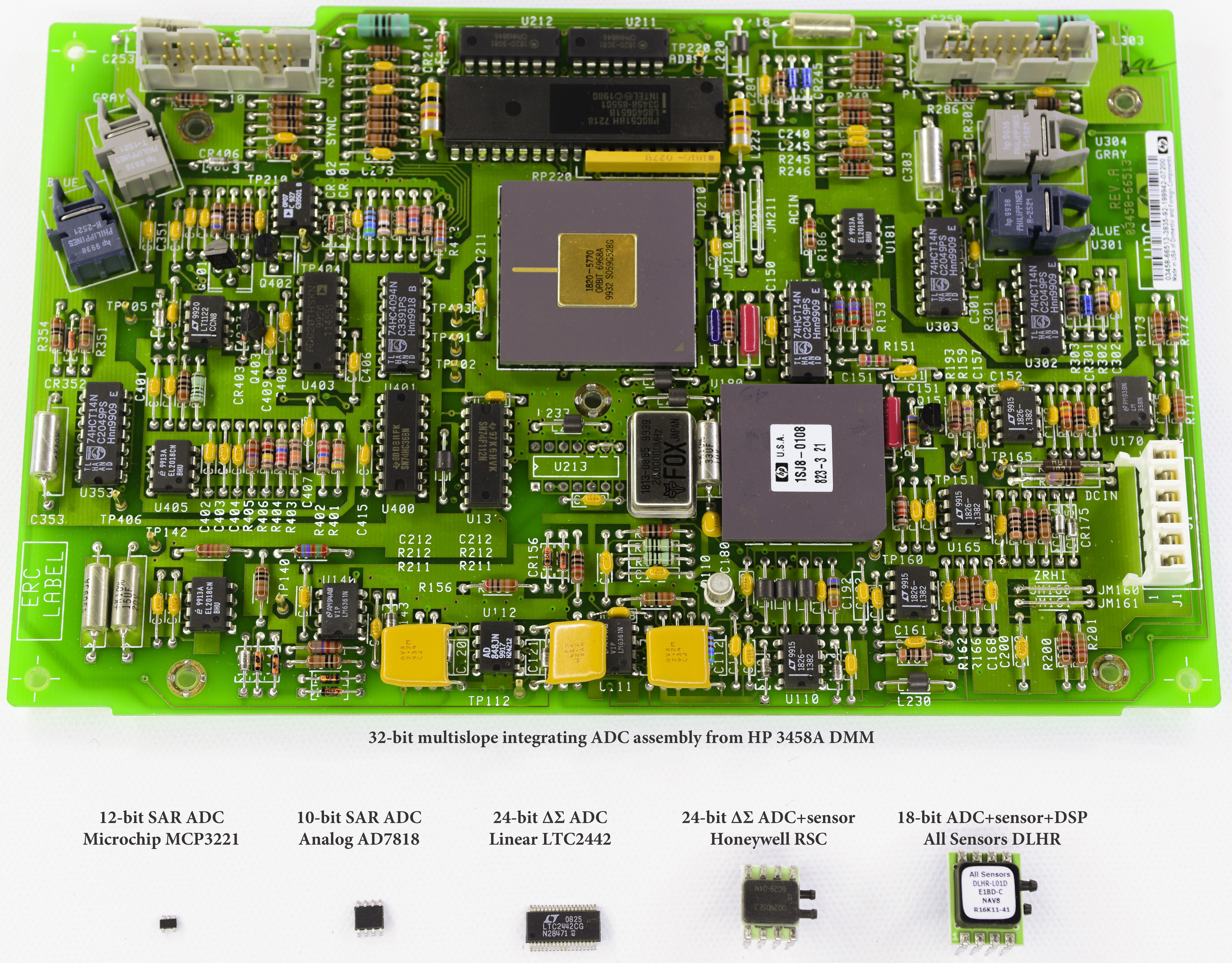
Image 3. Different packages and types of ADC designs
Easy to see from the Image 3, how complex high-resolution high-accuracy discrete ADC can be. High accuracy and stability require use of custom-made matched components in hermetic ceramic packages, expensive operational amplifiers, take lot of space and have number of control signals and power requirements to function. Today use of such precise integrating ADC in electronics are limited to narrow niche applications, where cost and design footprint are less important that performance. One of such examples are 6½-digit+ multimeter, paired with discrete high-stability references or instrumentation applications. SAR and high-resolution ΣΔ ADC solutions got closer in performance to state of the art multi-slope integrating ADC, replacing them in many designs due to much smaller package options, ease of use and affordable cost.
Now we know how to convert voltage from sensor into digital code, and as result know how to convert analog pressure into digital code. Practical demonstration of using such design covered in next section using integrated sensor hybrid, which have both analog sensor and ADC components inside same compact package.
Overview on pressure sensor design and construction
To demo pressure sensor and application in electronic device, I’ve got few modern sensors to perform some experiments and measurements. These sensors can be bought from usual retailers such as DigiKey or Mouser in single quantities. Table below shows acquired sensors and their key specifications.
| Sensor | Typical accuracy | Product page |
|---|---|---|
| All Sensors DLHR-L10D | ±0.25% | URL |
| All Sensors DLHR-L02D | ±0.25% | URL |
| All Sensors DLHR-L01D | ±0.25% | URL |
| Honeywell RSCDRRM020NDSE3 | ±0.25% | URL |
| Honeywell RSCDRRI002NDSE3 | ±0.5% | URL |
Table 6. Pressure sensors with digital front-end selected for test
Also worth to have a brief look on key specifications.
| DLHR-L10D | DLHR-L02D | DLHR-L01D | RSCDRRM020NDSE3 | RSCDRRI002NDSE3 | |
|---|---|---|---|---|---|
| Pressure range | Diff., ±10 inH2O | Diff., ±2 inH2O | Diff., ±1 inH2O | Diff., ±20 inH2O | Diff., ±2 inH2O |
| Sensor die configuration | 5-resistor bridge, 2×2mm proprietary die | 4-resistor bridge, 2.5×2.5mm proprietary die | |||
| ADC Type | 16/17/18-bit Δ-Σ | 24-bit Δ-Σ TI ADS1220 | |||
| Accuracy, FSR | ±0.25% | ±0.25% | ±0.5% | ||
| Output rate | 15 to 270 SPS | 20 SPS to 2000 SPS | |||
| INL | ±15 ppm of FSR (ADC) | ||||
| PSRR,CMRR | Unknown | PSRR 80dB+, CMRR 90dB+, 95dB@50/60Hz (ADC) | |||
| Power requirements | Single, 1.68 – 3.63 VDC | Single, 2.3 – 5.5 VDC | |||
| Onboard temperature sensor | Yes, 16 bits | Yes, 14 bits | |||
| Temperature range | -25°C to +85°C | -40°C to +85°C | |||
| Digital interface | I2C, SPI | SPI | |||
| One off reference price (DigiKey/Mouser) | $53.04 USD | $57.61 USD | |||
Table 7: Specification comparison of used pressure sensors
As we can see, disregarding output data resolution, accuracy specifications are same, except low pressure RSCDRRI002NDSE3 sensor, which specified for worse ±0.5% FSR. This confirms earlier theory, that accuracy of the pressure sensor is a system measure, not depending on ADC resolution.
For ±10 inH2O pressure sensor available digital resolution of 15 bits meaning pressure resolution tiny 0.00061 inH2O. Of course this is great sensitivity, but it does not really show the complete story, as output sensor accuracy specified at ±0.25%, which is full 40.96 bits (calculated as 0.25% * RangeFS / LSB). Thus sensor linearity, gain stability and complete accuracy are often more concerning factors for pressure measurement application.
Also there is no benefit increasing ADC resolution without redesign of sensor and signal conditioning front end to match with lower input noise level requirements. This is what limits availability of very low pressure sensors, due to noise from amplifier gain dominates own ADC input-referred noise. As result input gain stage and sensor bridge noise must be improved to allow lower noise to make higher ADC resolution useful. Methods to increase resolution by reducing sampling speed and performing more averaging/filtering have own limits as well due to 1/f noise components, and can provide only up to 2-3 bits extra.
All sensors pressure devices internal design
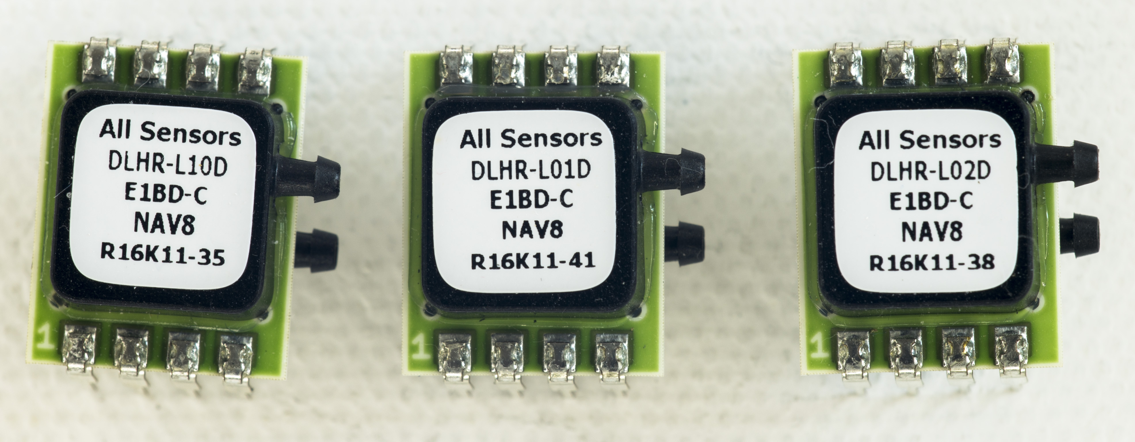
Image 4. All Sensors DLHR-type 18-bit pressure sensors
All of these sensors are differential type, best suited for low pressure levels. This is one of most challenging applications, as low-pressure sensors affected by common mode errors and offset. Especially interesting will be to evaluate if extra resolution available from digital domain translate to less noisy pressure reading. These calibrated and compensated sensors provide accurate, stable output over a wide temperature range. These sensors are designed for use with non-corrosive, non-ionic working fluids such as air, dry gases. All sensors also have protective parylene coating for moisture/harsh media as option.
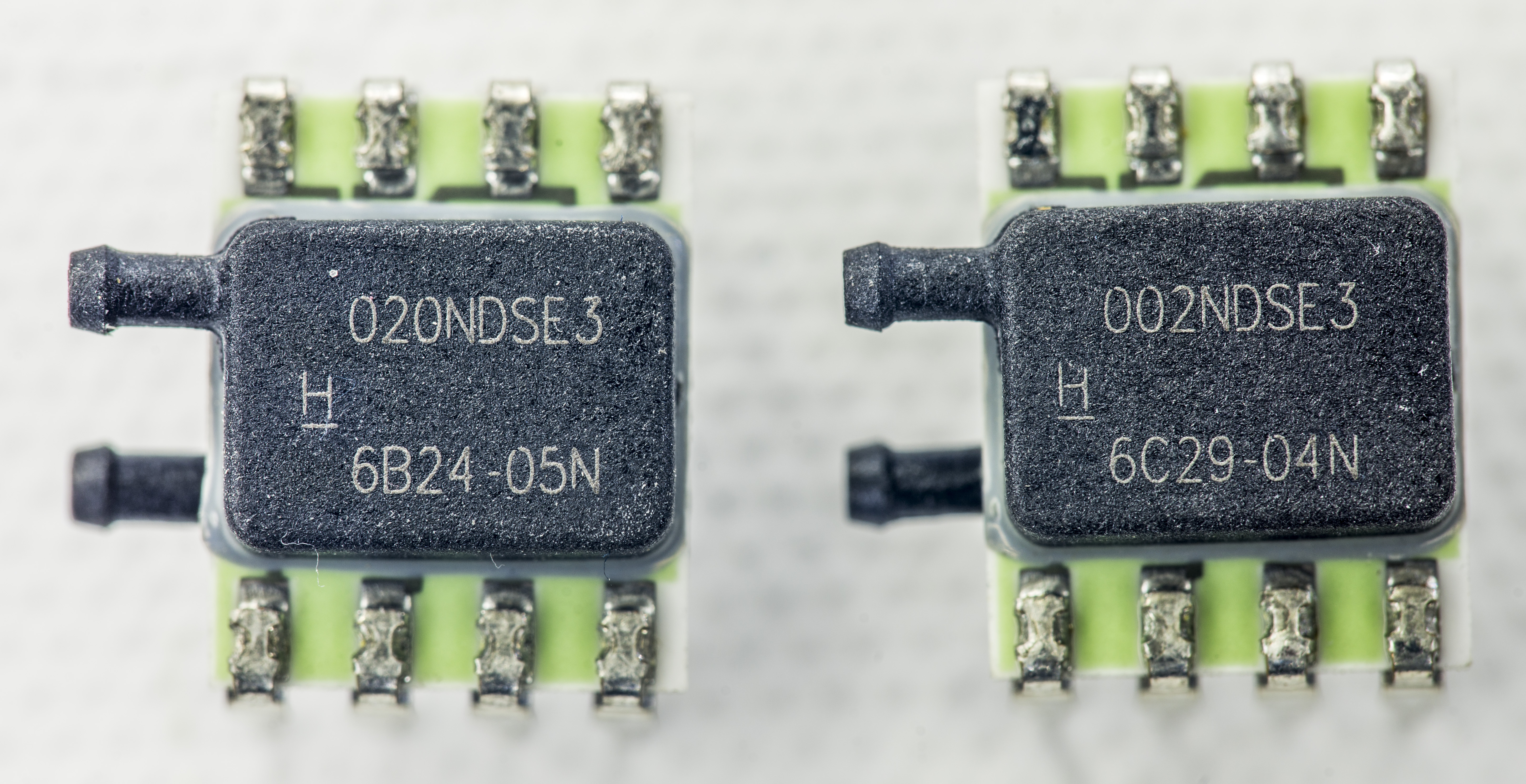
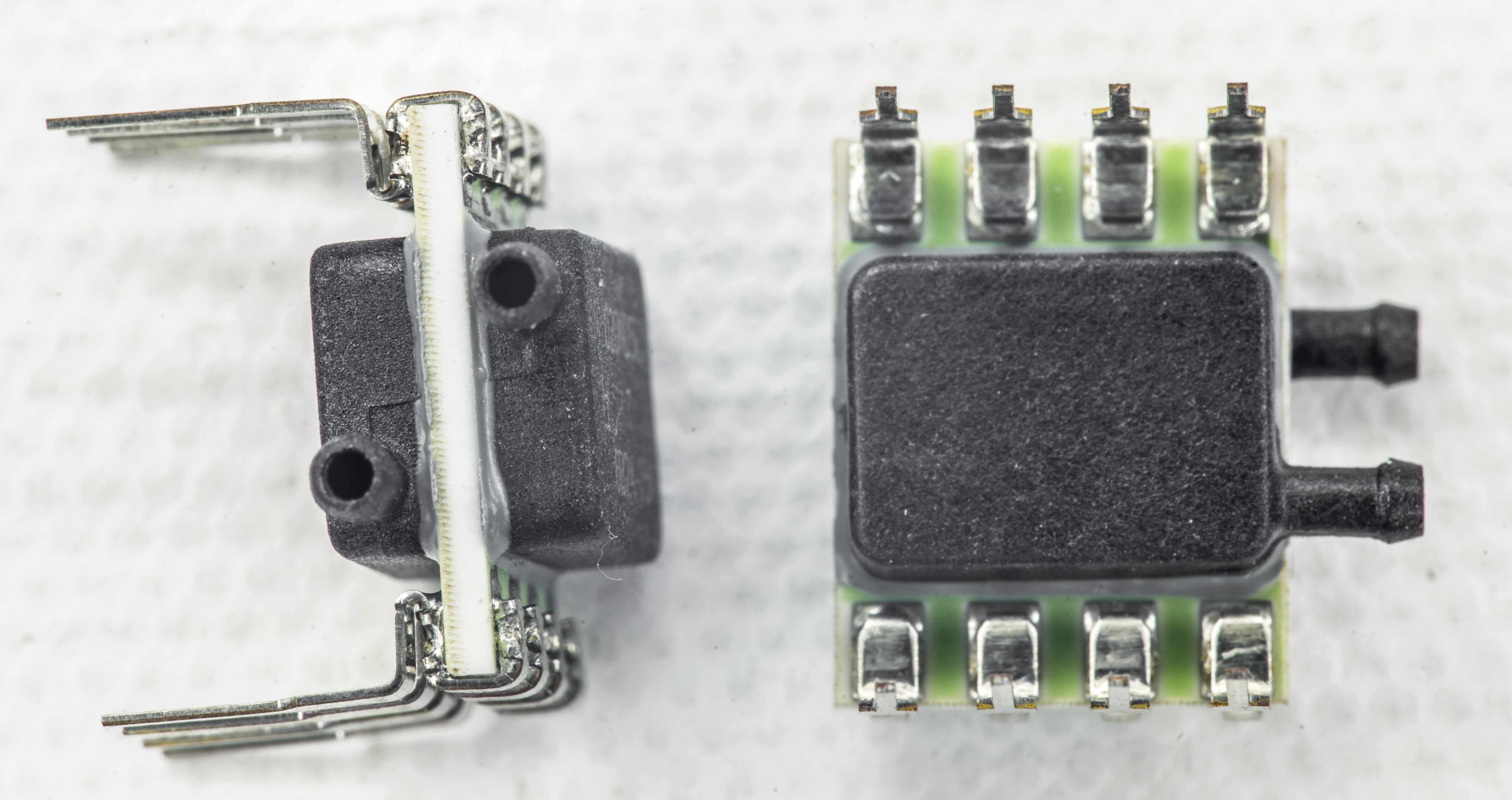
Image 5-6. Honeywell RSC differential 24-bit pressure sensors
These sensors are already equipped with internal mixed signal ASIC, containing ADC, voltage reference, current bias circuitry to excite sensor bridge elements, digital interface logic and calibration memory. There is also temperature sensor, which is crucial to obtain accurate pressure readouts. Pressure measurement errors depend heavily also on sensor die temperature, so onboard temperature sensor used to correct errors from temperature variations.
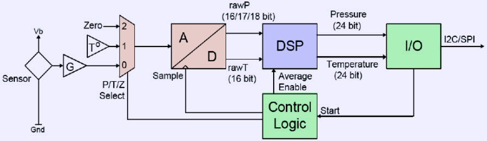
Image 7. ASC DLHR sensor internal block diagram
Quite a lot going on in this sensor. From left to right, pressure bridge sensor signal is routed through multiplexer into amplifier and further converted by ADC into digital code. Digital code resolution is set by sensor SKU, and processed by on-board DSP ASIC. Additional channels of same multiplexer/ADC path are used to obtain temperature reading and zero reference for compensation and calibration purposes. Interface block and control is responsible of getting data in and out, as well as providing trigger and sync for the system.
All this functionality in a same package allow easy and quick integration of sensor into your specific design. However this comes at price, as sensors with digital readout are more expensive. For battery-powered systems, the sensor also has low power mode between readings to minimize load on the power supply.
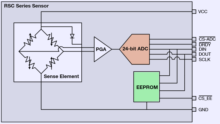
Image 8. Honeywell RSC internal block diagram
Honeywell’s sensor is bit simpler, having only analog domain converter and EEPROM with manufacturer-written calibration data. So it needs host controller to perform calibration and correction math. Calibration constants are stored in sensor’s EEPROM and readable by same SPI interface, just using separate chip select line. Both pressure readings must be compensated and corrected, depends on die temperature.
There are also simpler sensors available on the market, for smaller cost. However total solution implementation using analog sensor require higher engineering cost, increased complexity of design and more board space. Design and validation of accurate bridge analog front-end, ADC, current bias and compensation circuitry require significant effort, and in the end may be inferior to all-in-one digital pressure sensor. Such approach often viable only in large scale product manufacturing or with special specification requirements for particular application.
For educational purposes number of faulty analog sensors was taken apart to study their design and construction.
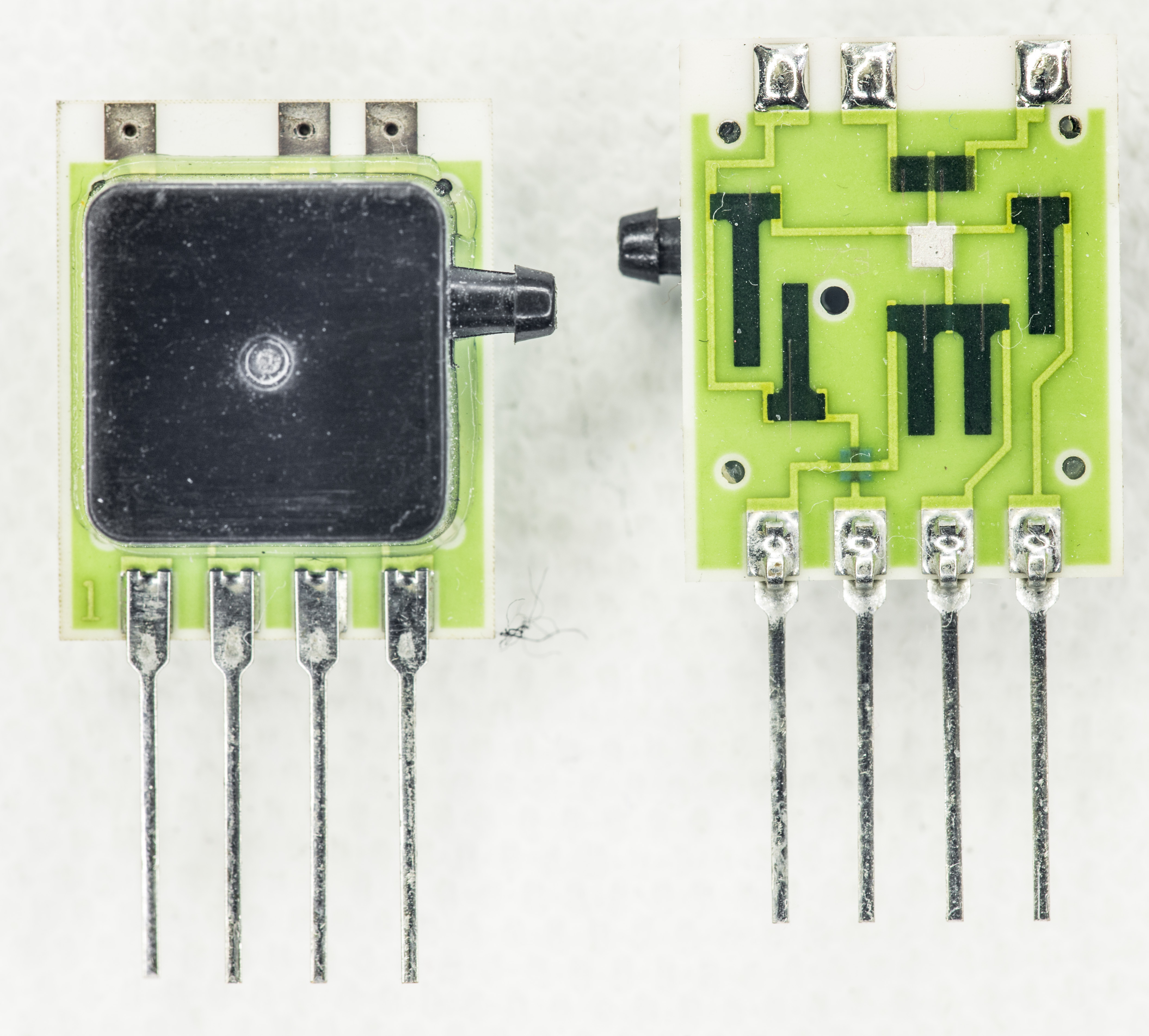
Image 9. Simpler All sensors analog sensor
Transducer design on photo above does not have digital or interfacing logic. Other than sensor die, there are only trimming/linearization resistors embedded on bottom side of alumina substrate. Alumina ceramics material as module substrate for it’s great humidity resistance and mechanical strength. Standard FR4 material greatly suspected to air humidity changes, and in application like pressure sensor humidity can easily cause a disaster. Pressure sensor die can detect even tiny stress changes, and FR4 flexibility may cause unwanted stress from baseboard PCBA into sensor. That would convert pressure sensor into assembly quality sensor, not what usual design engineer looking for.
Good eye can catch laser trim marks on dark resistor films. That meaning calibration and offsets correction to some extent for each manufactured sensor.
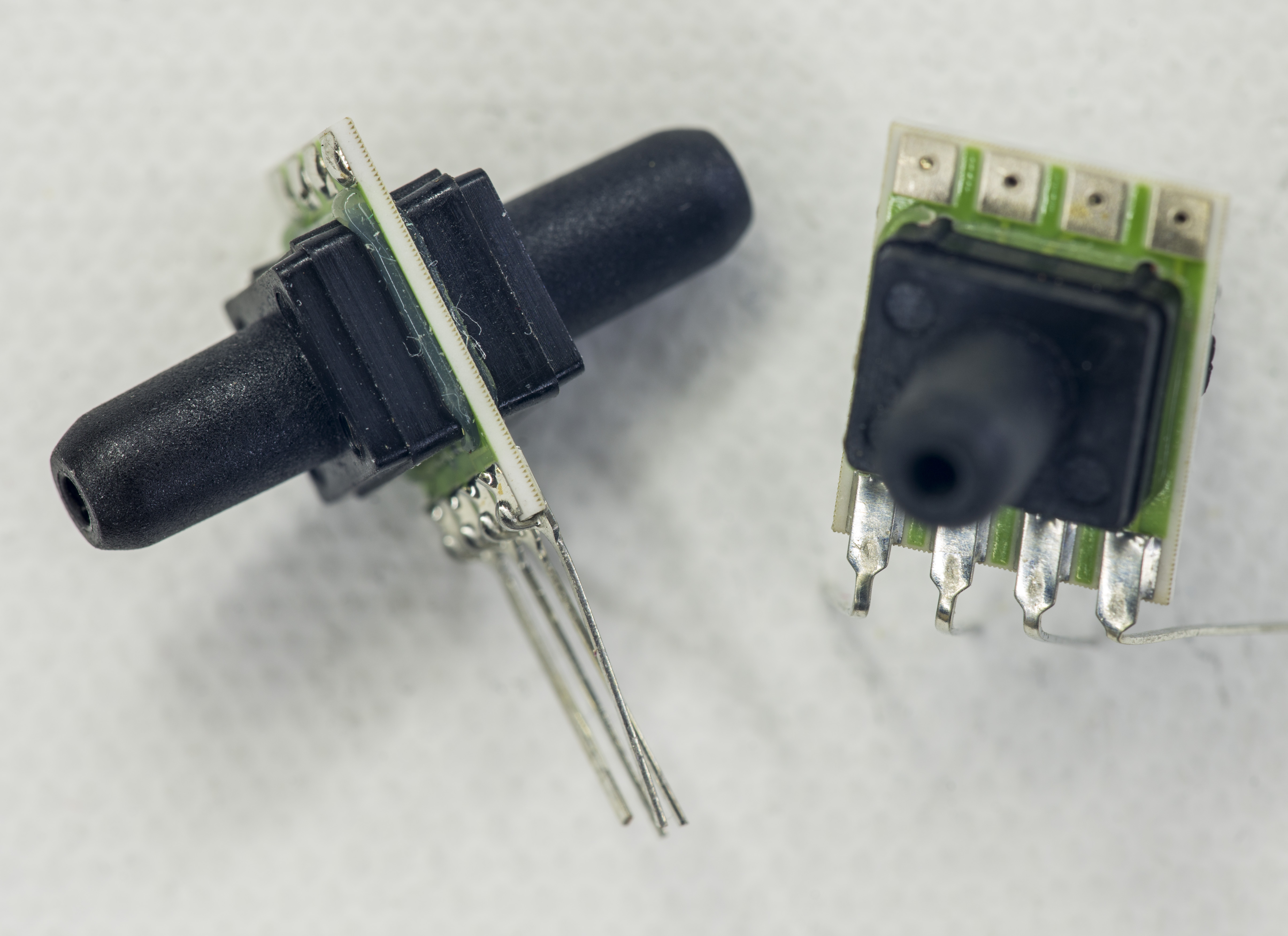
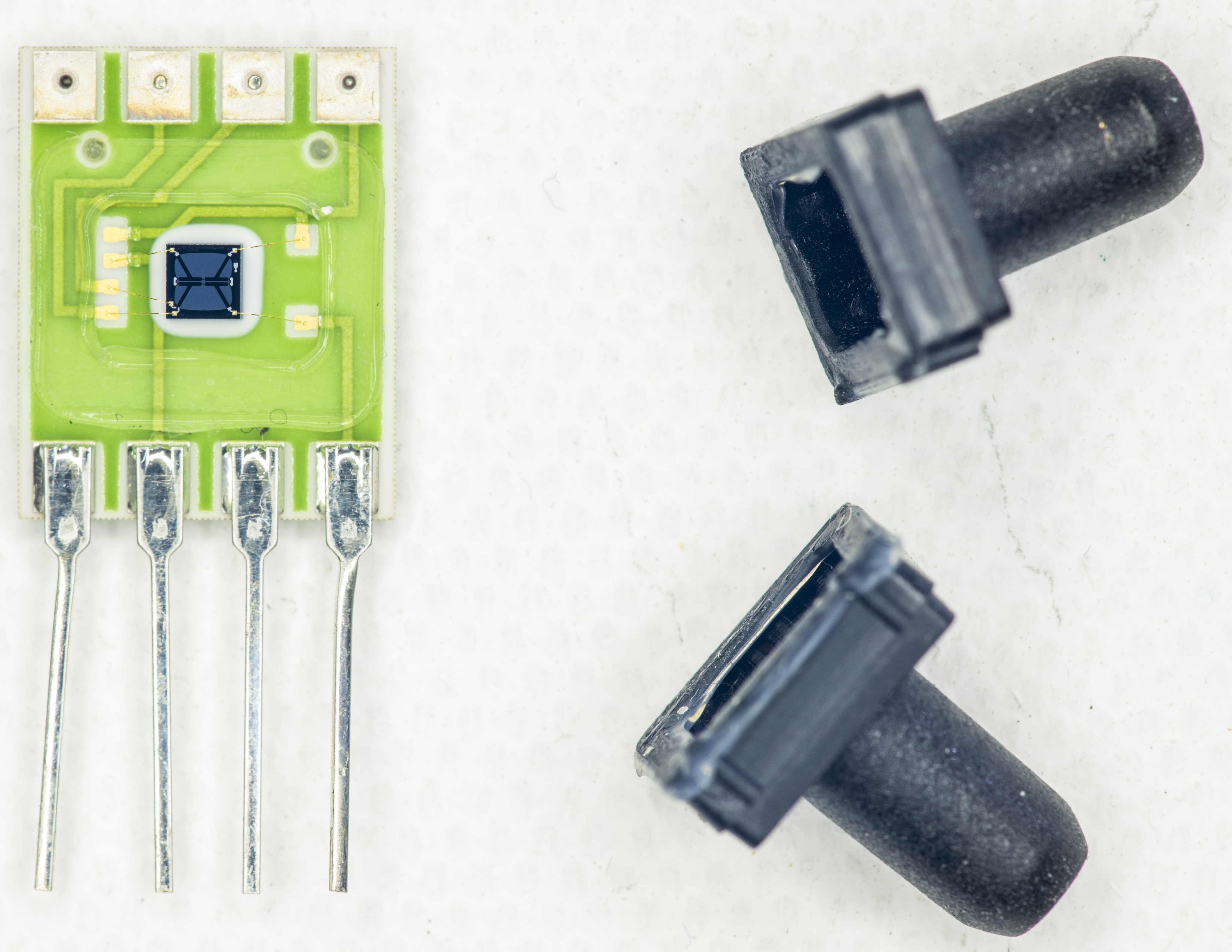
Image 10-11. Differential analog pressure sensor
Differential pressure sensors have two cavity ports, available in multiple mechanical configurations and types. When you order specific sensor pay attention to type of ports, as order code and part number is different depends on design. Alumina substrate and sensor die itself are same across family.
Some of the sensors come with rugged plastic or even metal chassis. This fits demanding applications well, providing additional level of mechanical and electrical protection to fragile ceramic substrate and compensation circuitry. Also larger case allows integration of additional electronics, making possible custom-made pressure transducers for specific customer needs. Let’s crack one open to see one inside?
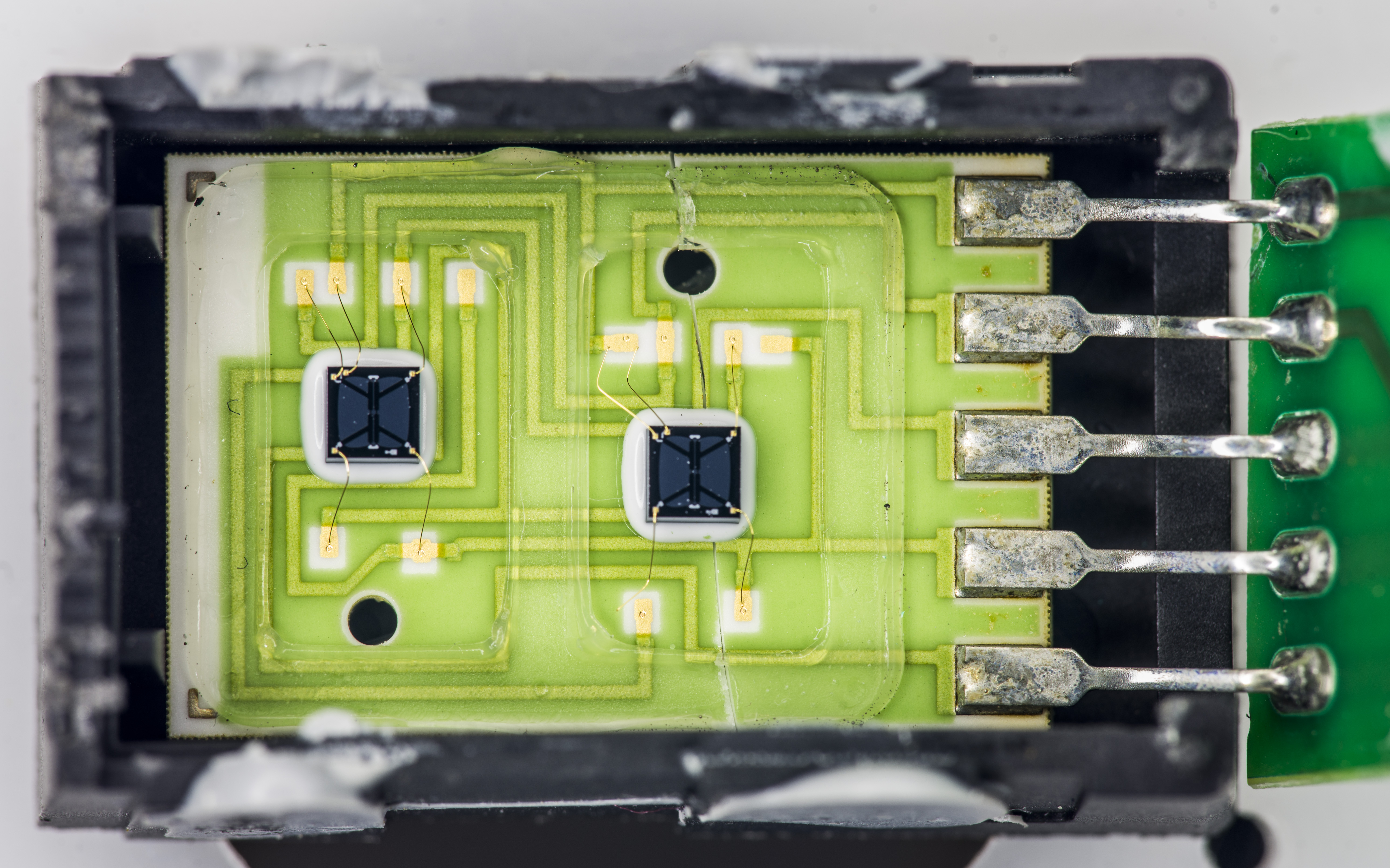

Image 12-13. All Sensors differential sensor in CASE-A enclosure
This is still analog sensor without analog/digital conversion or interface logic, but here are two pressure sensor die. Why two? It’s not easy to compensate silicon die for good accuracy, linearity and stability. Instead of spending all the effort to make a perfect sensor on single die, All Sensors made alternative choice to use two of the same sensor dies, route pressure to them in opposite direction, and measure differential signal between the two.
Since silicon die from same batch have good correlation, errors such as non-linearity, temperature dependence and offsets can be nulled from the output signal. In simple words such arrangement is similar idea to making Wheatstone bridge from two on-die bridge sensors. This method is patented (US6023978) as to provide active dual-die compensation for common mode pressure sensor errors.
Let’s have a closer look on sensor die itself.
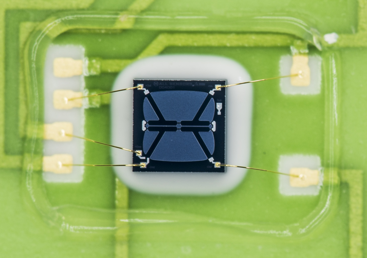
Image 14. ASC Pressure sensor die
With bit of magnification actual die marking are visible, revealing D04D01 and All Sensors 2009 marking. Bit more magnification also reveals die signal pad names, such as Vs+ (bridge supply input), +Gnd, -Gnd, -Out and +Out. Two grounds and separate resistor provided for compensation reasons.
Sensor is based around piezoresistive structure with special configuration silicon die. Square 2 × 2 mm die have cavity integrated on bottom side, right under the sensing element. Die structure used in All Sensors chip uses a proprietary Collinear Beam2 Technology registered as COBEAM2™. This technology provides better performance, especially for low pressure measurements. COBEAM2™ Technology designed to provide better pressure sensitivity in small package, which previously required boss structures and larger die topologies. Smaller die design without boss structure significantly reduce both unwanted gravity and vibration sensitivity.
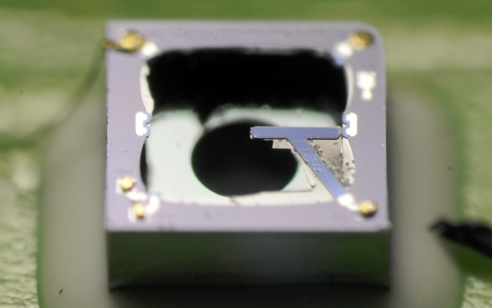
Image 15. Damaged membrane sensor with visible cavity area
Laser trimmed film resistors on alumina substrate are adjusted to improve linearity and accuracy of the sensor output. Each sensor has unique trim to provide calibrated and specified output. Using one of dead sensors as test vehicle, measurement of temperature coefficient of such surface resistors was performed. Sensor die was disconnected by removing the bond wires, so purely passive resistance could be measured.
| Tested resistor | Nominal value at +24 °C | TCR | Graph |
|---|---|---|---|
| R5 | 308.5885 KΩ | -13.24 ppm/°C | 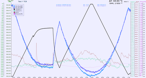 |
| R6 | 274.3273 KΩ | -12.37 ppm/°C | |
| R7 | 152.09743 Ω | -52.12 ppm/°C | 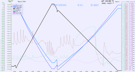 |
| R8 | 149.20517 Ω | -55.13 ppm/°C |
Table 8. All Sensors embedded film resistors TCR matching test
Temperature coefficient measured in range from +24 °C to +57 °C. Results show that compensation resistors are matched well <5 ppm/°C and overall resistance ratio maintained stable even with large temperature variation.
All Sensors Eval board review
All Sensors evaluation kit targeted for testing pressure sensors, before the prototype design process. This evaluation kit is capable of providing data on digital, millivolt, and amplified pressure sensors and have following features:
- ZIF socket allows instant electrical connection, without need of soldering or pin forming.
- Display data from Digital sensors in one of 12 convenient units
- Capture data from Digital sensors to CSV text file, with sample index and timestamp on each readout
- Uses standard Windows USB HID drivers. Eval board using micro-USB connector for data/power.
- Standard 4mm “banana”-type terminals for lab test equipment and external power
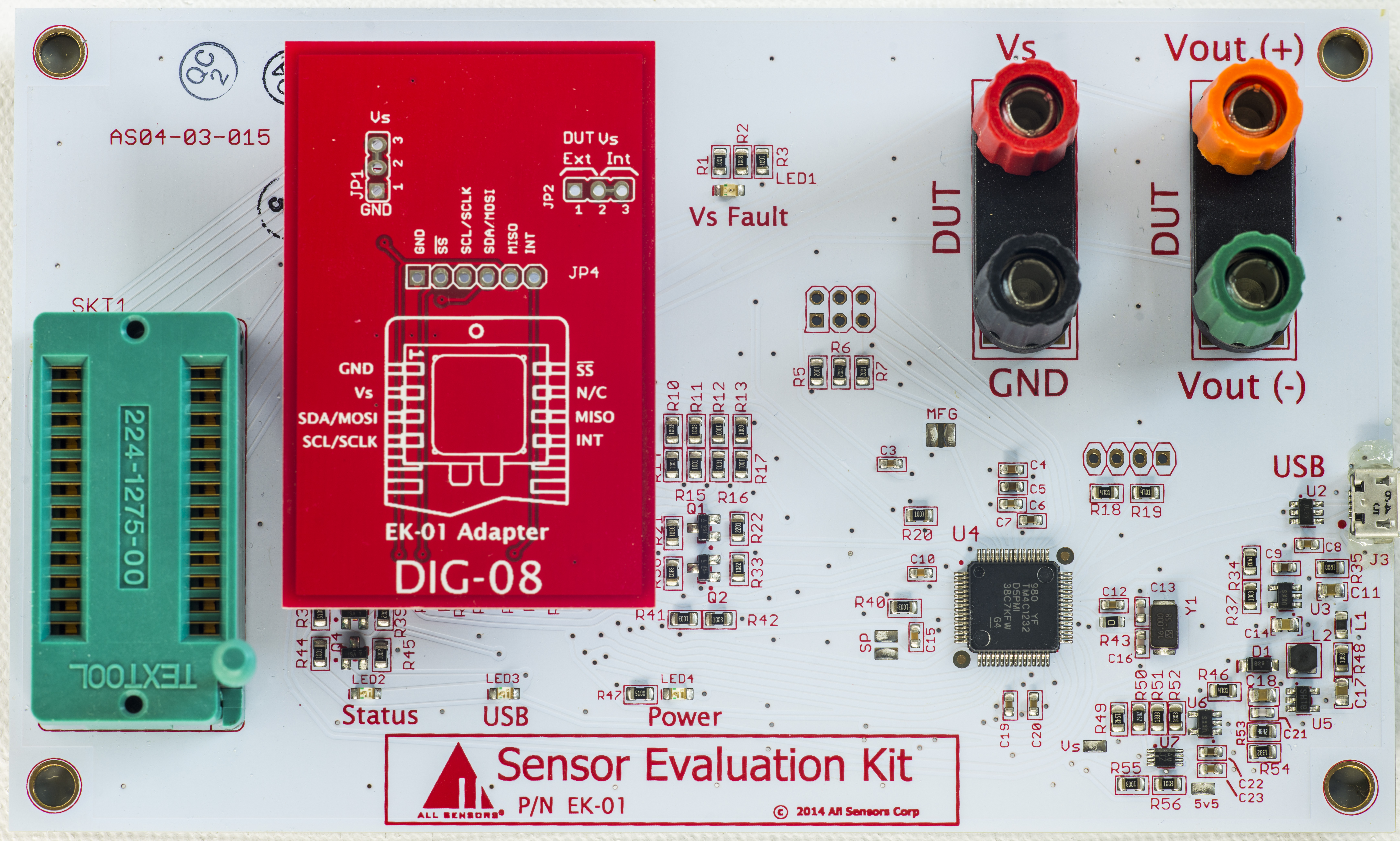
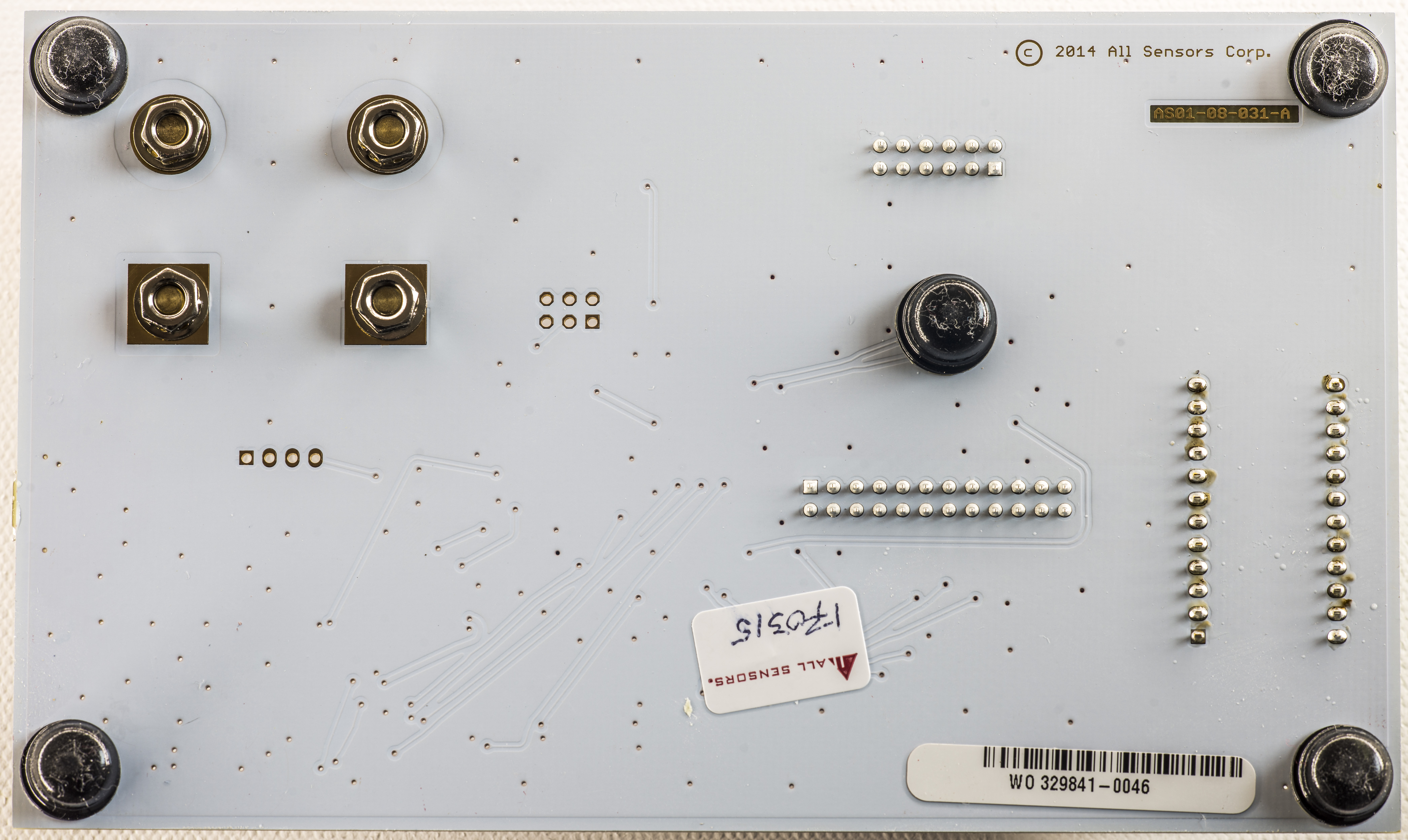
Image 16-17. Evaluation board for All Sensors devices
Evalkit based around Texas Instruments TM4C1233D5PM Cortex-M4F ARM® microcontroller. It has native USB 2.0 interface, I2C and SPI interfaces to talk with sensors and specified to operate in industrial range.
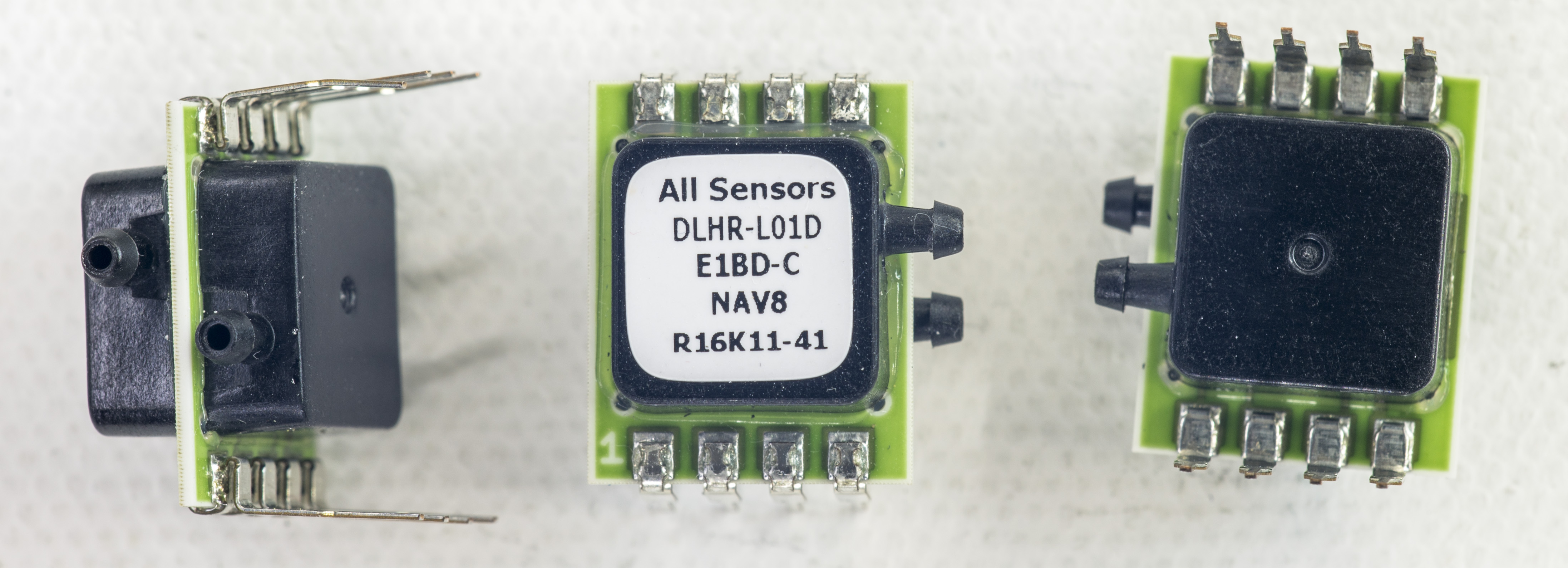
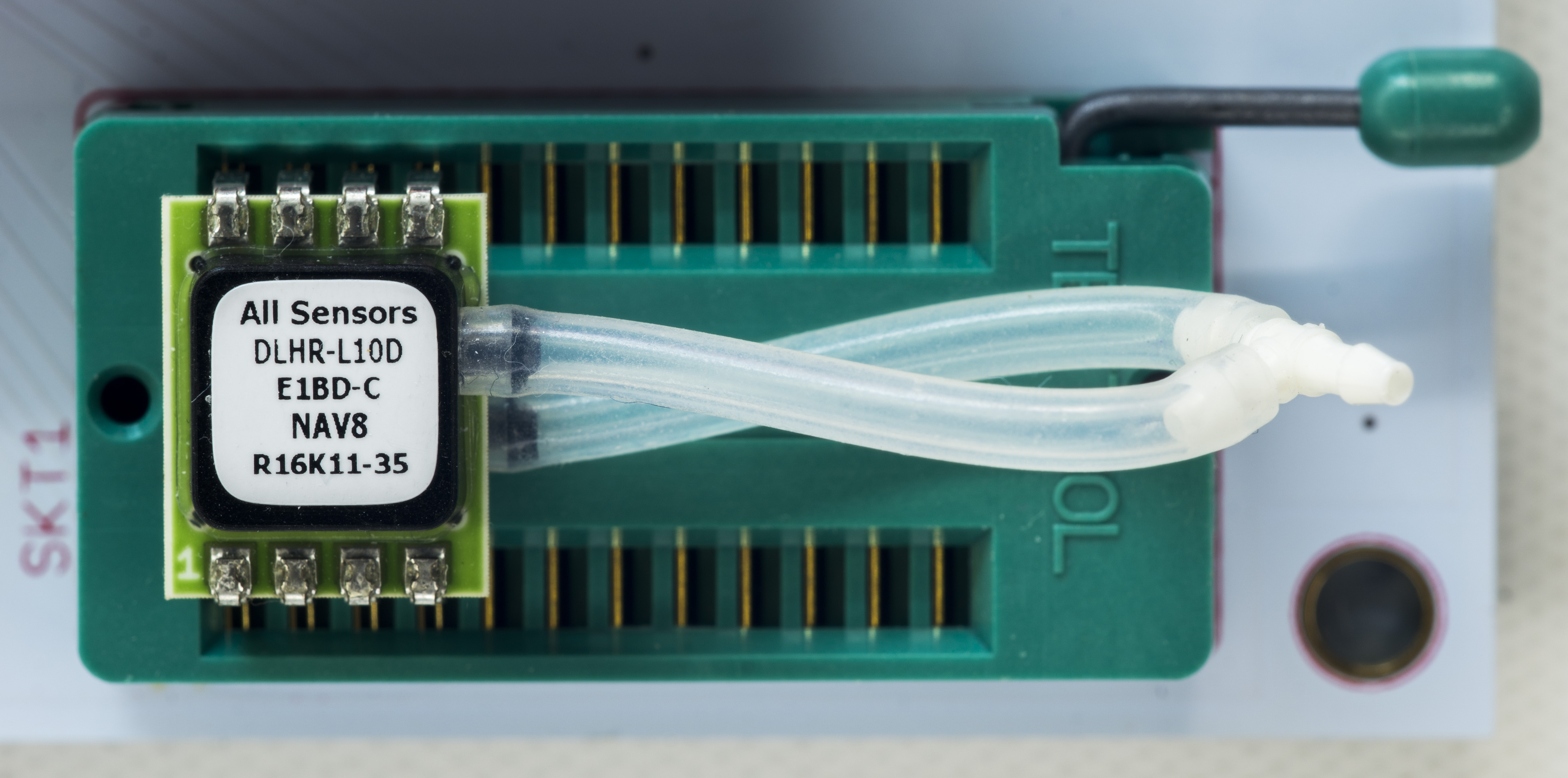
Image 18-19. Sensor and connection to Evalboard socket
Evaluation kit comes with simple to use software tool. It supports various sensors with both SPI and I2C interface connections, and can be used to set data timings, pressure units and average filtering power. Once sensor properly configured, software reads both pressure and temperature and display result on GUI. Storage into CSV file can be used for longer data captures and external data analysis.
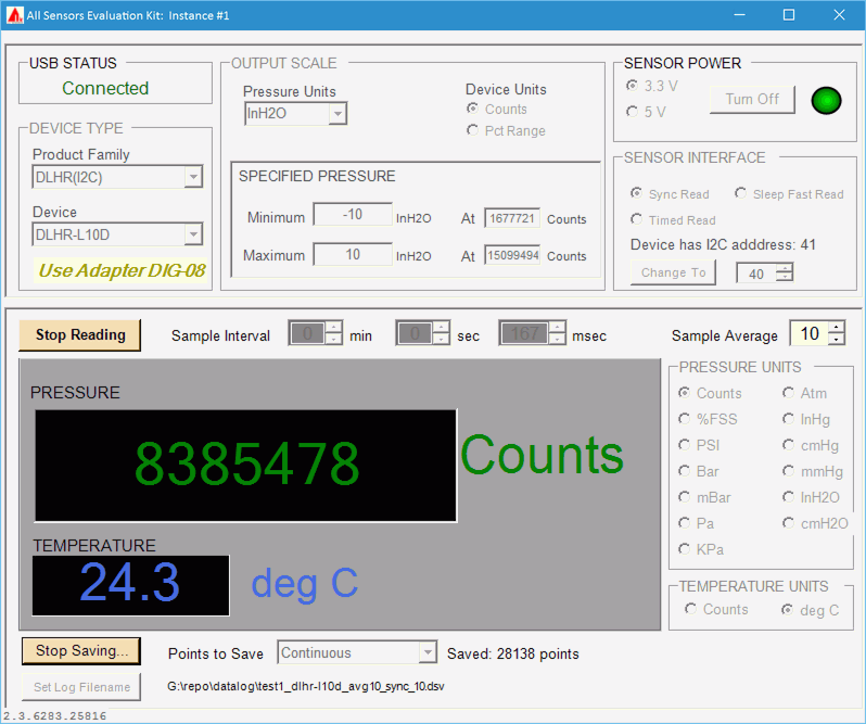
Image 20. Demo kit software GUI
Honeywell RSCDRRM020NDSE3 sensor design
After sample data collection was complete, one of Honeywell RSC sensors was disassembled to find out what’s hidden inside. Just like All Sensors design, circuit implemented on alumina carrier. After decapping three semiconductor components were found.
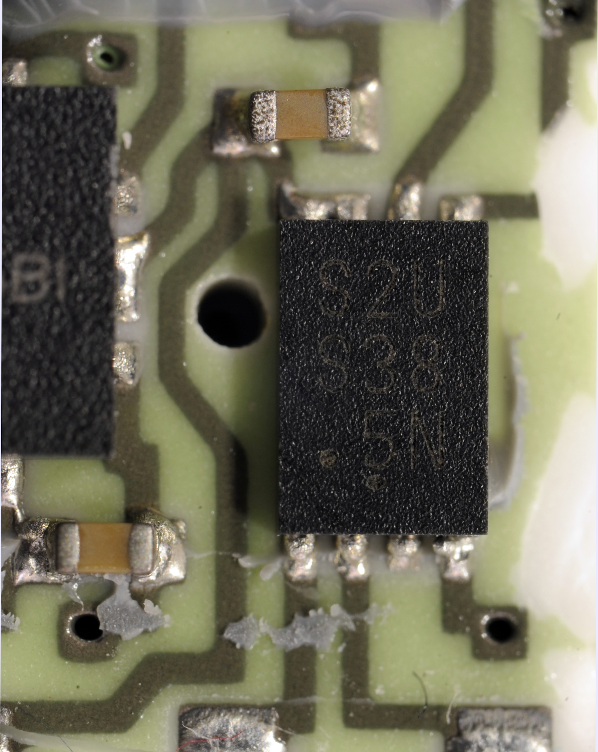

Image 21-22. RSC sensor ROM and ADC ICs
Top side have just two ICs, which are Texas Instruments ADS1220 24-bit ΔΣ ADC, with speed up to 2KSPS and integrated PGA, voltage reference and precision temperature sensor. ADC have 4 input channels, perfectly suitable for pressure sensor bridge measurements. Programmable 10 µA-1.5mA current source which is crucial for bridge operation is also present. TI’s 1g Resolution over 15kg Range Front-End Reference Design covering use of ADS1220 with bridge sensors very well. Tiny DFN16 package makes integration of this ADC on compact sensor carrier easy task, without need of additional wire bonding.
Also being able to identify ADC chip leaves us with full register information, so perhaps one can even play with different currents/filter modes to tune pressure sensor operation. Of course there would be no warranty or support from Honeywell, if you do so. :)
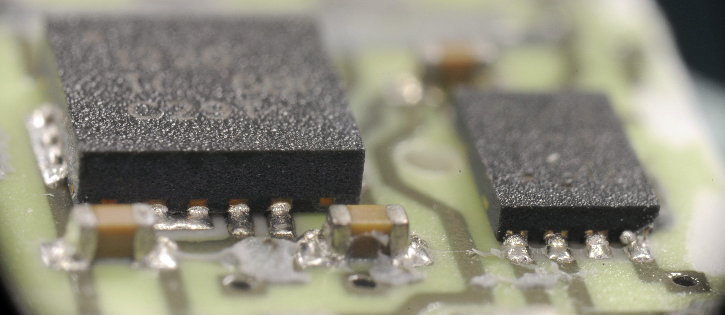
Image 23. DFN packages soldered to alumina substrate pads
Smaller chip next to ADC is DFN8-packaged CAT25040HU4I-GT3 4Kbit SPI EEPROM. Nothing very special about it. We can also see pressure port to sensor die cavity, it’s a hole right between EEPROM and ADC. Time to look on the sensor itself.
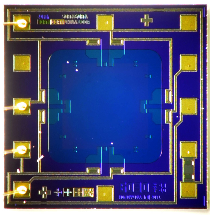
Image 24. Honeywell RSC pressure sensor die
Sensor die marked as Honeywell 6030 and have design year 2011. Label next to 6030 state X-17 Y-10, probably meaning sensor element center position? Four piezoresistors located on the middle points of membrane edges. Membrane boundary can be easily seen by eight fiducial marks around. Die size is 2.5 × 2.5 mm.
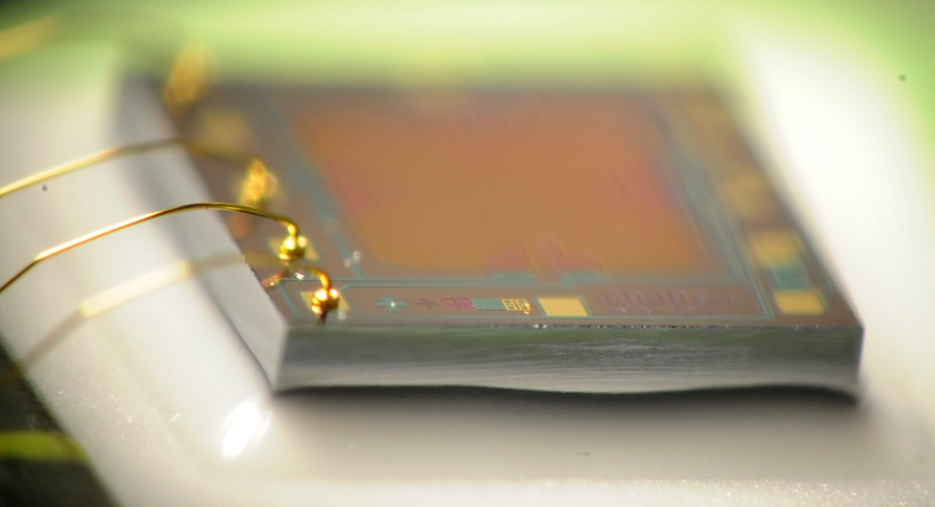
Image 25. Die attach sealant
Die bonded with semitransparent white adhesive, as it’s important to maintain hermetic connection between alumina base and bottom of the sensor, where cavity port is located.

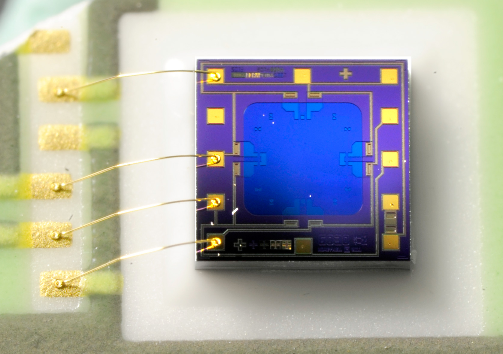
Image 26-27. Sensor structures and bridge piezoresistve assembly
Purple-colored area is flexible section, with membrane visible in smaller box inside. Note two different resistor die configuration, used in the bridge. There is nothing else on the sensor, outside borders of the die just have some lot/batch cryptic code markings and etching test/alignment structures.
Based on RSC product page site development kit based on Arduino Uno board. User Instructions how to connect everything, firmware for it and example source code available in Software Download sections.
Test setup and methodology
To demo interfacing and operation of both DLHR-LxxD and RSC sensors popular single-board computer platform, such as Raspberry Pi 3 Model B chosen as development environment. This is well known Linux-based platform, with wide recognition in education, scientific labs and multitude of various application projects, including even industrial field. Raspberry Pi have set of different interfaces, including I2C and SPI, that can be used will to talk with sensors. Integrated networking functionality, ability to output image using standard HDMI port and rich Linux-based software toolkit allow quick and efficient prototyping and testing new ideas.
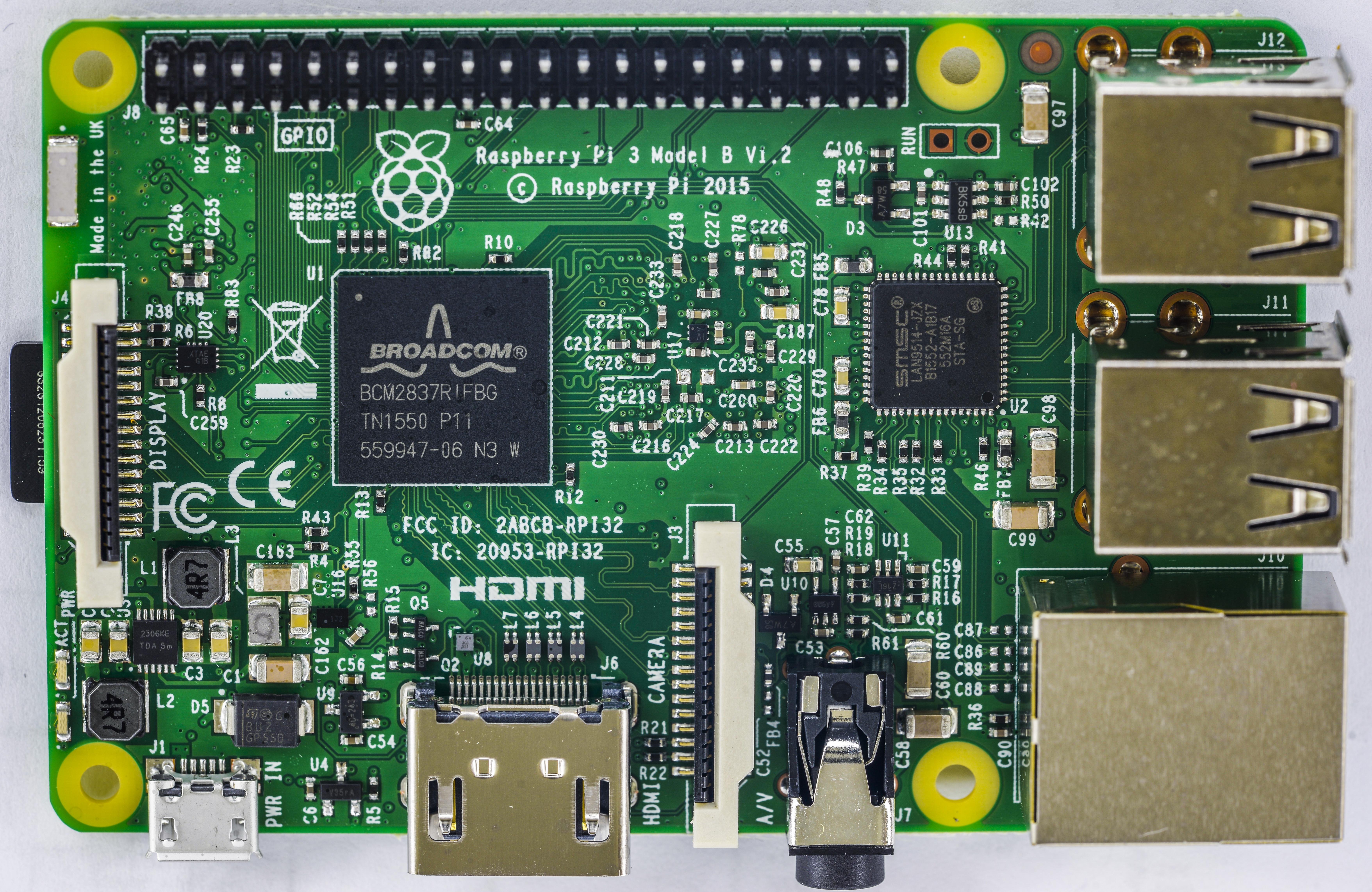
Image 28. Raspberry Pi 3 Model B used for test
In our case Pi will interface pressure sensor interface (I2C in case of ASC DLHR-LxxD and SPI for Honeywell RSC), configure them and sample both temperature and pressure data into local SD-card filesystem. All data will be tagged with datestamp and stored in DSV-format for further math processing. Language of choice for the measurement experiments is Python 2.7.
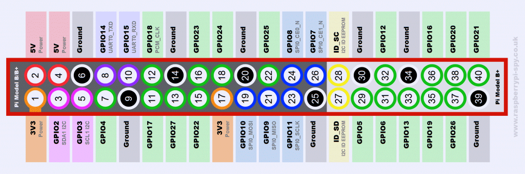
%(imgref)Image 29. RPI3 Pinout. Courtesy of www.raspberrypi-spy.co.uk
Since I had no means to generate different pressures for test, I’ve bought Fluke 719 30G portable pressure calibrator. It has integrated pressure pump, pressure sensor and 4-20mA current loop source/measure capability. This is commonly used tool for industrial applications, where pressure transducers required to be tested and calibrated. 719 30G model with electrical pump can source pressures in range from -850 mbar (-341 inH2O) to 2.4 bar (963 inH2O), with resolution of 0.1 mbar (0.0401 inH2O).
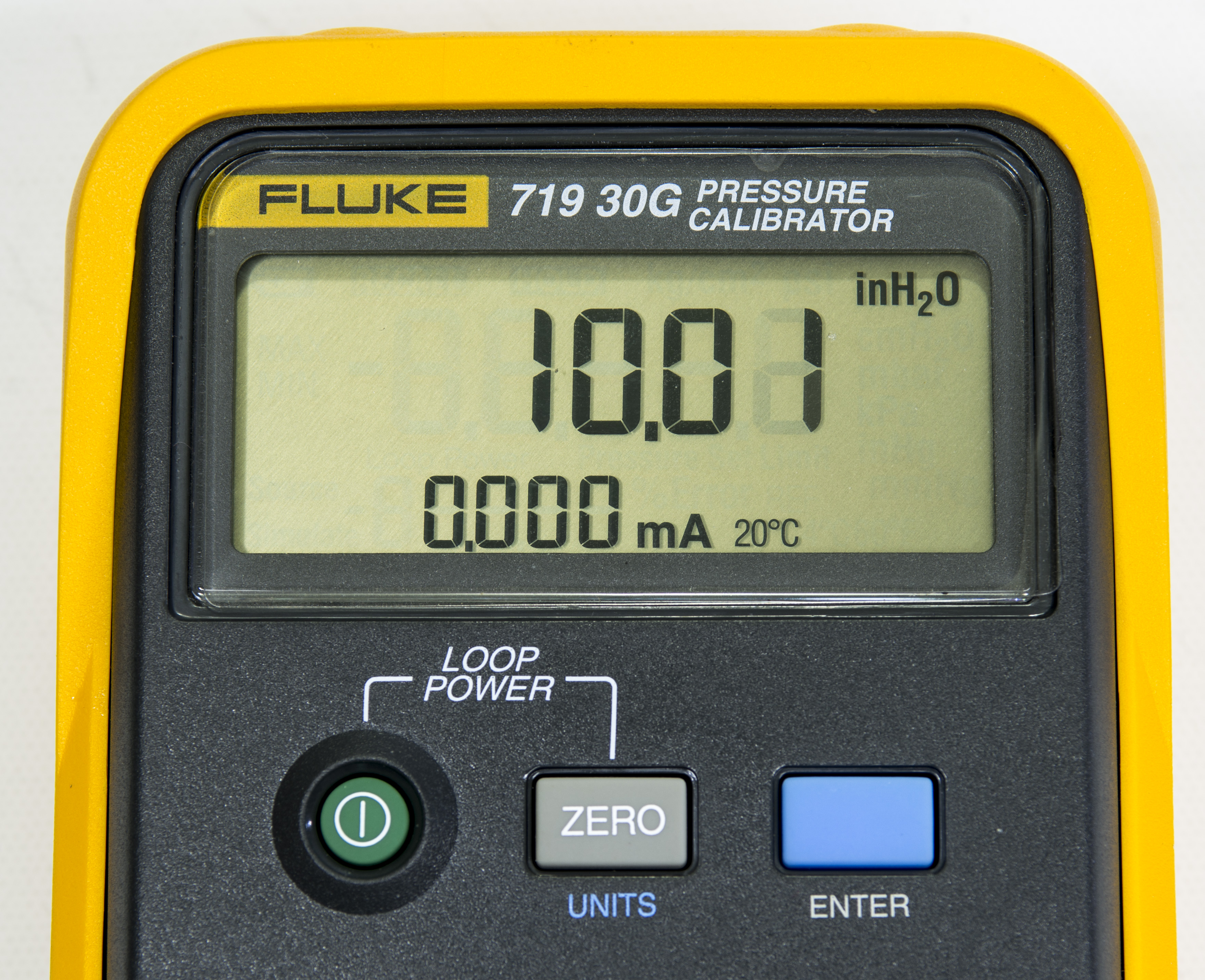
Image 30. Fluke 719 30G electric pressure calibrator
Best accuracy over a year is 0.035%, sufficient for testing our sensors, which are specified around 0.25%. Fluke 719 Manual covers operation and functions of calibrator. Detailed specifications also provided in the manual.
Now that we have pressure source and reference meter, time to get back figuring out how to connect sensor to the Raspberry Pi. Datasheets for both sensors have all the information required. DLHR sensors in ND package have following pinout:
| Pin number | Pin function | Body | Pin function | Pin number |
|---|---|---|---|---|
| 1 | GND (Ground reference) | /SS (chip select) | 8 | |
| 2 | VS Supply 1.65-3.6V | No connection | 7 | |
| 3 | SDA/MOSI Data interface | MISO SPI Data | 6 | |
| 4 | SCL/SCLK Clock | EOC status | 5 |
Table 9. All Sensors DLHR pinout
Honeywell RSC sensor also feature 8-pin package, with slightly smaller size.
| Pin number | Pin function | Body | Pin function | Pin number |
|---|---|---|---|---|
| 1 | SCLK Clock input | MISO SPI Data | 8 | |
| 2 | ~DRDY Data ready output | CS_ROM (Chip select for EEPROM) | 7 | |
| 3 | DIN/MOSI | VS Supply 1.65-3.6V | 6 | |
| 4 | CS_ADC (Chip select for ADC) | GND (Ground reference) | 5 |
Table 10. Honeywell RSC pinout
Reference connections also presented in datasheet, to that’s exactly what we do as well. Open-collector lines, such as SDA/SCL and chip-selects on RSC sensor need to be pulled up to power level for proper operation. This was done using 2.2 KΩ 1206-size SMT resistors connected to VS lines.
Both sensors are powered by low-noise LDO converter. It is based on Linear LT3042EDD, very low noise adjustable linear regulator, capable of supplying enough current to run sensors. Great PSRR and RMS noise of this regulator help to reduce input noise coupling with our DUT.
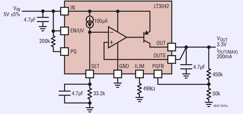
%(imgref)Image 31. Typical LT3042 regulator application. (Courtesy Linear
As LT3042 have compact SMT package, to make it easier for prototyping I’ve developed and assembled few adapter boards with onboard ceramic capacitors and resistors per reference schematics. Output voltage range is from 0V to 15V. Capacitor from SET to GND improves noise, PSRR and transient response at the expense of increased start-up time. For best load regulation, Kelvin connect the ground side of the SET pin resistor directly to the load point.
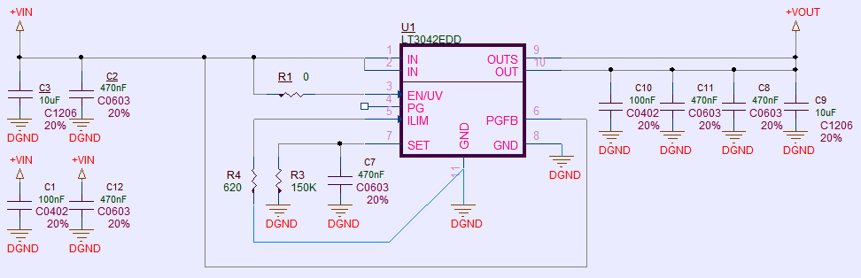
Image 32. xDevs.com LMP1 Power supply regulator schematics (resistor R3 set for +15V output as example)
Output voltage is set by resistor R3, connected at Pin 7 (SET). This pin is the inverting input of the error amplifier and the regulation set-point for the LT3042. Pin have fixed current source 100µA, so single resistor allows to set desired output voltage. Calculated output and resistance formulas presented as below.
VOUTPUT = 100µA * RSET, or RSET = VOUTPUT / 100µA
Adapter board allow simple three terminal operation and assembly of regulator on typical 0.1” breadboard. Adapter module is designed for same size and pinout as TO-220 78xx-series LDOs, using 4-layer FR4 PCB for all connections and ground copper pour.


Image 33-34. xDevs.com LMP1 module comparison to 7805 TO-220 regulator
Latest Raspberry Pi Linux distributive used as software platform with Python 2.7 development environment. Python is often a tool of choice for scientific and educational use, since it has easy syntax, have powerful functionality and comes with vast open-source library/API repository from developers community. Even people who never saw Raspberry Pi or Python can start and get first application running in matter of few evenings with tea and a laptop. All demo application code and test data presented in this article.
Connection map of sensors to Raspberry Pi I/O port is listed in table below.
| Pressure sensor pin | Signal type | Direction | Raspberry Pi pin |
|---|---|---|---|
| ASC DLHR pin 1 | GND (Ground reference) | Power | |
| ASC DLHR pin 2 | VS Supply 1.65-3.6V | Power | |
| ASC DLHR pin 3 | SDA/MOSI Data interface | Bidir | Pin 3 |
| ASC DLHR pin 4 | SCL/SCLK Clock | From Pi3 | Pin 5 |
| HW RSC pin 1 | SCLK Clock input | From Pi3 | Pin 23 |
| HW RSC pin 3 | DIN/MOSI | From Pi3 | Pin 19 |
| HW RSC pin 8 | MISO SPI Data | To Pi3 | Pin 21 |
| HW RSC pin 4 | CS_ADC (Chip select for ADC) | From Pi3 | Pin 24 |
| HW RSC pin 7 | CS_ROM (Chip select for EEPROM) | From Pi3 | Pin 26 |
| HW RSC pin 2 | ~DRDY Data ready output | To Pi3 | Pin 7 |
| HW RSC pin 6 | VS Supply 1.65-3.6V | Power | |
| HW RSC pin 5 | GND (Ground reference) | Power |
Table 11. Sensors interfacing to Raspberry Pi 3
Interfacing pressure sensors to Raspberry Pi using Python
Example libraries and demo application was developed in Python for testing both sensors. This allows for easy and quick way to integrate All Sensors transducers for IoT field and applications. Source code and example test data can be cloned from GitHub repository.
# git clone https://github.com/tin-/ascp
Also application have one additional sensor, Bosch BME280, used to log environment conditions, such as atmosphere pressure, relative humidity and temperature. Guide about using this sensor was already covered on xDevs.com.
Directory structure have just few main files:
- main.py – Top level application code, contains menu, help prompts and module imports.
- dlhr.py – Have low-level and math for All Sensors DLHR type sensor.
- rsc.py – Have low-level and math for Honeywell RSC type sensor.
- bme280.py – Have low-level and math for Bosch BME280 environment sensor.
- pressure.conf – Configuration file for settings
This application depends on few external modules, which need to be installed in user’s Python environment:
- Adafruit_GPIO.I2C – Provide binding to Pi I2C port to Python
- spidev – Provide binding to SPI device in Python
- RPi.GPIO – Provide binding to Pi GPIO port to Python
- ConfigParser – Provide configuration file parsing
Take a brief look on used functions..
dlhr.py – All Sensors DLHR sensor module.
This module have all necessary functions to interface I2C with DLHR sensor, read/write all necessary data and expose high-level functions for application’s top level.
class ASC_DLHR(object):
    def __init__(self, mode=ASC_DLHR_I2CADDR, address=ASC_DLHR_I2CADDR, i2c=None,
                 **kwargs):
        self._logger = logging.getLogger('Adafruit_BMP.BMP085')
        # Check that mode is valid.
        if mode != 0x41:
            raise ValueError('Unexpected address'.format(mode))
        self._mode = mode

        # Create I2C device.
        if cfg.get('main', 'if_debug', 1) == 'false':
            if i2c is None:
                import Adafruit_GPIO.I2C as I2C
                i2c = I2C
            self._device = i2c.get_i2c_device(address, **kwargs)
Class ASC_DLHR creates I2C device and checks correct address.
def write_cmd(self, cmd):
        if cfg.get('main', 'if_debug', 1) == 'false':
            bus.write_i2c_block_data(ASC_DLHR_I2CADDR, cmd, [0x00, 0x00])
            time.sleep(0.1)
    if cfg.get('main', 'if_debug', 1) == 'true':
        print "\033[31;1mDebug mode only, command = %X\033[0;39m" % cmd,
        return 1
This function write command cmd into DLHR following protocol from datasheet on the sensor.
def chk_busy(self):
        if cfg.get('main', 'if_debug', 1) == 'false':
            Status = bus.read_byte(ASC_DLHR_I2CADDR)
        #Status = self._device.readRaw8()  # Receive Status byte
        if cfg.get('main', 'if_debug', 1) == 'true':
            Status = 0x40

        if (Status & ASC_DLHR_STS_BUSY):
            print "\033[31;1m\r\nPower On status not set!\033[0;39m",
            return 1 # sensor is busy
        return 0     # sensor is ready

This function checks sensor flag if conversion already done and data is available to read.
Test code to read sensor data below:
    def read_sensor(self):
        outb = [0,0,0,0,0,0,0,0]
        time.sleep(0.04)
        self.retry_num = 5
        while self.retry_num > 0:
            if self.chk_busy():
                print "\033[31;1m\r\nSensor is busy!\033[0;39m",
                time.sleep(0.01)                       # Sleep for 100ms
            else:
                self.retry_num = 0
            self.retry_num = self.retry_num - 1

        outb = bus.read_i2c_block_data(ASC_DLHR_I2CADDR, 0, 7)
        StatusByte = outb[0]

        # Check for correct status
        if (StatusByte & ASC_DLHR_STS_PWRON) == 0:
            print "\033[31;1m\r\nPower On status not set!\033[0;39m",
            quit()
        if (StatusByte & ASC_DLHR_STS_SNSCFG):
            print "\033[31;1m\r\nIncorrect sensor CFG!\033[0;39m",
            quit()
        if (StatusByte & ASC_DLHR_STS_EEPROM_CHKERR):
            print "\033[31;1m\r\nSensor EEPROM Checksum Failure!\033[0;39m",
            quit()

        # Ccnvert Temperature data to degrees C:
        Tmp = outb[4] << 8
        Tmp += outb[5]
        fTemp = float(Tmp)
        fTemp = (fTemp/65535.0) * 125.0 - 40.0

        # Convert Pressure to %Full Scale Span ( +/- 100%)
        Prs = (outb[1] <<16) + (outb[2]<<8) + (outb[3])
        Prs -= 0x7FFFFF
        fPress = (float(Prs))/(float(0x800000))
        fPress *= 100.0

        print "Status: 0x%X " % StatusByte,
        print "\033[35;1mPressure: %4.5f %%FSS \033[33;1m Counts: %d " % (fPress, (outb[1] <<16) + (outb[2]<<8) + (outb[3]) ),
        print "\033[36;1mTemperature: %3.3f 'C \033[39;0m" % fTemp

    with open('asc_dlhr.dsv', 'ab') as o:
        o.write (time.strftime("%d/%m/%Y-%H:%M:%S;")+('%4.5f;%3.3f;\r\n' % (fPress, fTemp)))
        return 0
Now these low level functions can be used to get sensor data.
print ("Reading AVG8 sensor Pressure/temp..\033[0;49m")
        sensor.write_cmd(ASC_DLHR_AVG8_READ_CMD)
        sensor.read_sensor()
rsc.py – Honeywell RSC sensor module.
Same idea used for Honeywell RSC sensor.
class HRSC(object):
    def __init__(self, i2c=None, **kwargs):
        self._logger = logging.getLogger('Adafruit_BMP.BMP085')
        # Create device.

    self.read_eeprom()
        # Load calibration values.
Class HRSC used to create SPI device and initialize sensor port
    def read_eeprom(self):
        print "Loading EEPROM data from sensor",
        print ".",
        # Assert EEPROM SS to L, Deassert ADC SS to H, Set mode 0 or mode 4
        spi.open(0, 1)
    spi.mode = 0b00
    for i in range (0,255):
        sensor_rom[i] = spi.xfer([HRSC_EAD_EEPROM_LSB, i, 0x00], 100000)[2] # Read low page
#        print "%c" % (sensor_rom[i]),
    for i in range (0,255):
            sensor_rom[i+256] = spi.xfer([HRSC_EAD_EEPROM_MSB, i, 0x00], 100000)[2] # Read high page
    # Clear EEPROM SS , set mode 1 for ADC
        spi.close()
        return 0
Function read_eeprom collects binary data from all 512 bits of sensor’s internal EEPROM.
def adc_configure(self):
        # Clear EEPROM SS , assert ADC SS, set mode 1 for ADC
    spi.open(0, 0)
        spi.mode = 1
    self.bytewr = 3
        self.regaddr = 0

        # Reset command
        test = spi.xfer([HRSC_ADC_RESET], 10000)
    time.sleep(1)
    # Write configuration registers from ROM
    print ("%02X" % sensor_rom[61]),
    print ("%02X" % sensor_rom[63]),
    print ("%02X" % sensor_rom[65]),
    print ("%02X" % sensor_rom[67]),
        test = spi.xfer2([HRSC_ADC_WREG|self.regaddr << 3|self.bytewr & 0x03, sensor_rom[61], sensor_rom[63], sensor_rom[65], sensor_rom[67] ], 10000)
        spi.close()
        return 1
Function adc_configure resets ADC and initialize it with correct configuration from ROM. Oscilloscope screenshot of this sequence and speed change shown below.
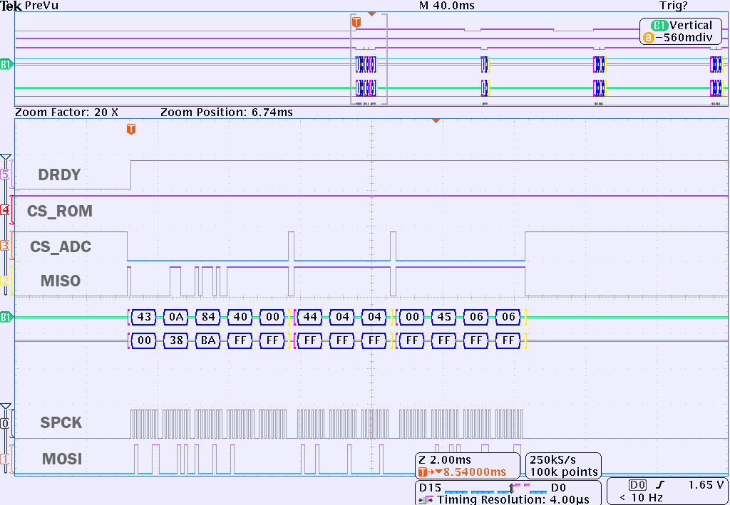
Image 35. Oscilloscope capture for ADC configuration. CH3 – CS_ADC.
    def sensor_info(self):
        # Check for correct status
        print "\033[0;32mCatalog listing : %s" % str(bytearray(sensor_rom[0:16]))
        print "Serial number   : %s" % str(bytearray(sensor_rom[16:27]))
        print "Pressure range  :",
        b = self.conv_to_float(sensor_rom[27], sensor_rom[28], sensor_rom[29], sensor_rom[30])
    print b,sensor_rom[27:31]
        print "Pressure min    :",
    b = self.conv_to_float(sensor_rom[31], sensor_rom[32], sensor_rom[33], sensor_rom[34])
    print b,sensor_rom[31:35]

    print "Pressure units  : %s" % str(bytearray(sensor_rom[35:40]))
        print "Pressure ref    :",
    if (sensor_rom[40] == 68):
        print "Differential"
        print "Checksum        :",
    b = self.conv_to_short(sensor_rom[450], sensor_rom[451])
    print b,sensor_rom[450:452]
        print "\033[0;39m"
    return 1
sensor_info using EEPROM data to print sensor’s partnumber, operation range, sensor type and it’s serial number.
def read_temp(self):
        # Clear EEPROM SS , assert ADC SS, set mode 1 for ADC
    spi.open(0, 0)
        spi.mode = 1
    self.bytewr = 0
        self.regaddr = 1
    spi.max_speed_hz = 10000

    reg_dr = 0
    reg_mode = 0 # 256kHz modulator
    reg_sensor = 1 # temperature
    self.reg_wr = (reg_dr << 5) | (reg_mode << 3) | (1 << 2) | (reg_sensor << 1) | 0b00
    # Write configuration register
    command = HRSC_ADC_WREG|(self.regaddr << 2)|(self.bytewr & 0x03)
    print ("\033[0;36mADC config %02X : %02X\033[0;39m" % (command, self.reg_wr))
        test = spi.xfer([command, self.reg_wr], 10000)

    twait = 0.0591
    while(1):
            time.sleep(twait)
        adc_data = spi.xfer([0,0,command, self.reg_wr], 10000)
        #print "RDATA = ",
        #print adc_data
        temp_data = (adc_data[0]<<16|adc_data[1]<<8|adc_data[2])
        self.convert_temp(temp_data)
    spi.close()
    return 1
Function read_temp issues command to obtain temperature reading and converts binary data from sensor into floating point temperature. Output resoluion of temperature is 0.03125 °C.
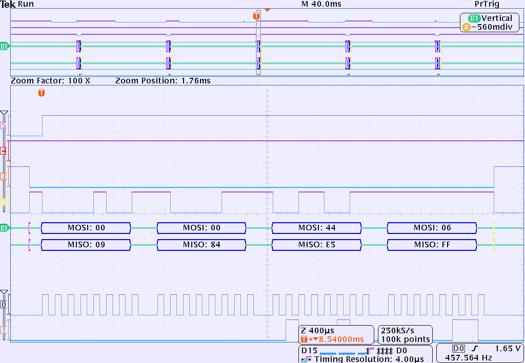
Image 36. Oscilloscope capture for temperature readout. MSB byte first.
def convert_temp(self, raw_temp):
    raw = (raw_temp & 0xFFFF00) >> 10
    if (raw & 0x2000):
        #print "MSB is 1, negative temp"
        raw = (0x3fff - (raw - 1))
        temp = -(float(raw) * 0.03125)
    else:
        #print "MSB is 0, positive temp"
        temp = (float(raw) * 0.03125)
        print "RAW: %s %s , %f" % (hex(raw_temp), hex(raw), temp )
    with open('rsc_temp.dsv', 'ab') as o:
        o.write (time.strftime("%d/%m/%Y-%H:%M:%S;")+('%4.5f;%3.3f;\r\n' % (0.0, temp)))
    return temp
Helper function convert_temp processes raw temperature binary value into floating point temperature, covering both negative and positive temperature ranges.
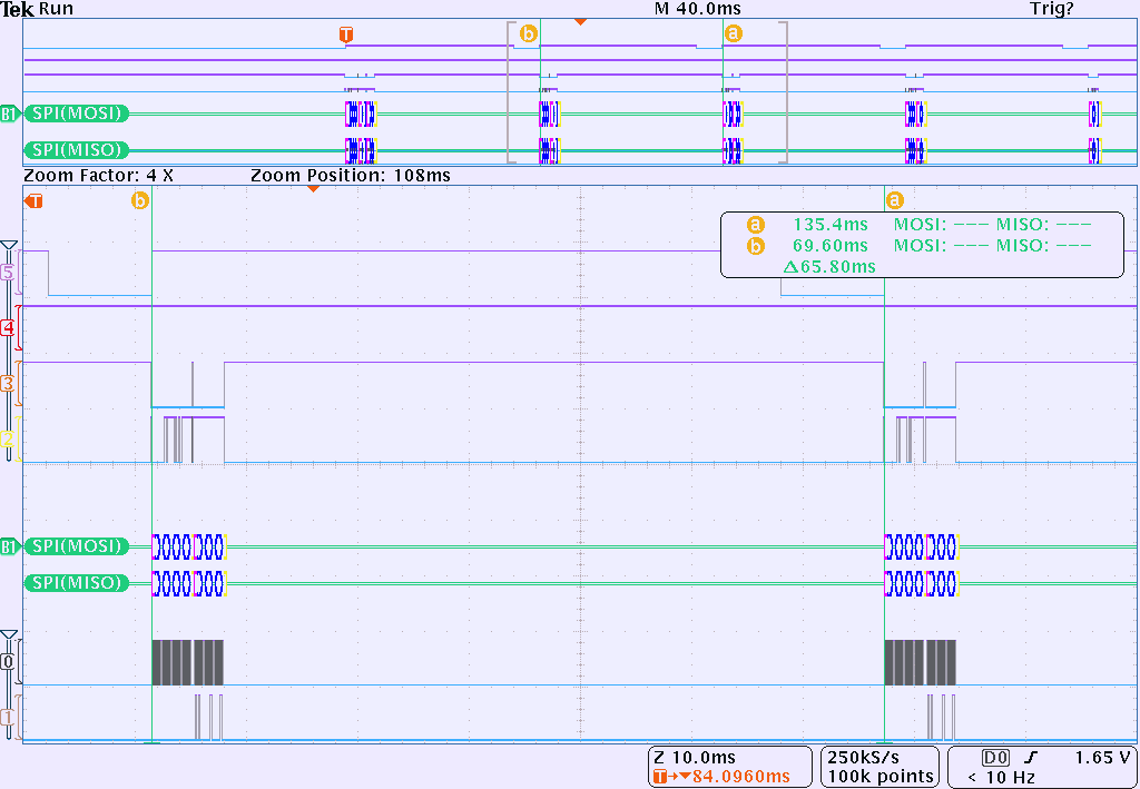
Image 37. Oscilloscope capture of timing between temperature readouts. CH5 – Data ready.
    def conv_to_float(self, byte1, byte2, byte3, byte4):
        import struct
    temp = struct.pack("BBBB", byte1,byte2,byte3,byte4)
    output = struct.unpack("<f", temp)[0]
        return output

    def conv_to_short(self, byte1, byte2):
        import struct
    temp = struct.pack("BB", byte1,byte2)
    output = struct.unpack("<H", temp)[0]
        return output
Helper functions conv_to_float and conv_to_short allow different formats conversion for user information prints
Example output of app menu
root@xdevs:/repo/ascp# python ./main.py
RSC sensor used
Running on   : Pi 3 Model B
Processor    : BCM2837
Revision     : a02082
Manufacturer : Sony
Loading EEPROM data from sensor .
  Pressure sensors toolkit CLI
  Using NI GPIB adapter and linux-gpib library
 Target platform: Raspberry Pi B 3+
********************************************************************************
[0] - Help guide
[1] - Detect instruments
[2] - Initialize instruments
[3] - Select DUT
[4] - Run PT procedure on DUT
[5] - Do performance test and autogenerate HTML report
[6] - Generate HTML report
[7] - a: Read part Pressure & Temp
[8] - b: Read part 2x oversampled Pressure & Temp
[9] - c: Read part 4x oversampled Pressure & Temp
[10] - d: Read part 8x oversampled Pressure & Temp
[11] - e: Read part 16x oversampled Pressure & Temp
[12] - U: Toggle Warmup cycles on/off
[13] - Test RSC sensor
[X] - Quit
Entering command number will trigger application to run specific task. For example menu item 13 will check communication with Honeywell sensor over SPI bus and collect some test data to check if readings are correct.
Testing RSC
1. Read the ADC settings and the compensation values from EEPROM.
Catalog listing : RSCDRRM020NDSE3
Serial number   : 20163220025
Pressure range  : 40.0 [0, 0, 32, 66]
Pressure min    : -20.0 [0, 0, 160, 193]
Pressure units  : inH2O
Pressure ref    : Differential
Checksum        : 38343 [199, 149]

2. Initialize the ADC converter using the settings provided in EEPROM.
0A 84 40 00 3. Adjust the ADC sample rate if desired.
4. Command the ADC to take a temperature reading, and store this reading.
ADC config 44 : 06
RAW: 0xc5e2b 0x317 , 24.719
RAW: 0xc5e69 0x317 , 24.719
RAW: 0xc5efd 0x317 , 24.719
RAW: 0xc5e8d 0x317 , 24.719
root@voltnut-xdevs:/repo/ascp#
Here’s SPI Honeywell RSC 002ND output test data.
********************************************************************************
Logging start..
Catalog listing : RSCDRRI002NDSE3
Serial number   : 20163620021
Pressure range  : 4.0 [0, 0, 128, 64]
Pressure min    : -2.0 [0, 0, 0, 192]
Pressure units  : inH2O
Pressure ref    : Differential
Checksum        : 25643 [43, 100]

   -2000 ASC:8379072;31.746 RSC:62983;33.312 A 33.448 R 40.97 P 1012.33 TEC:39.312 SV: 23.000
   -1999 ASC:8379328;31.769 RSC:63017;33.344 A 33.465 R 40.97 P 1012.36 TEC:39.301 SV: 23.000
   -1998 ASC:8379456;31.809 RSC:63016;33.344 A 33.477 R 40.98 P 1012.34 TEC:39.290 SV: 23.000
   -1997 ASC:8379584;31.788 RSC:63073;33.344 A 33.486 R 40.98 P 1012.34 TEC:39.279 SV: 23.000
   -1996 ASC:8379392;31.801 RSC:63009;33.375 A 33.497 R 40.98 P 1012.31 TEC:39.266 SV: 23.000
   -1995 ASC:8379136;31.855 RSC:63067;33.406 A 33.513 R 40.98 P 1012.38 TEC:39.257 SV: 23.000
   -1994 ASC:8379136;31.836 RSC:63089;33.406 A 33.523 R 40.98 P 1012.32 TEC:39.240 SV: 23.000
   -1993 ASC:8379456;31.878 RSC:63148;33.406 A 33.532 R 40.98 P 1012.36 TEC:39.232 SV: 23.000
   -1992 ASC:8379392;31.857 RSC:63110;33.438 A 33.541 R 40.99 P 1012.32 TEC:39.222 SV: 23.000
   -1991 ASC:8379840;31.914 RSC:63159;33.469 A 33.555 R 40.99 P 1012.30 TEC:39.208 SV: 23.000
Overview of sensors on test board in temperature test box.
Both All Sensors and Honeywell sensors are to be tested in same conditions, same time, using prototyping board with 100 mils pad spacing.
Each DUT connected to board using high-quality collect-type sockets. Interface lines are routed outside to Raspberry Pi. Power for whole setup except RPI3 provided by onboard linear regulator, which powered from Keithley 2400 SMU.
Sensor test board placed in metal die-cast box with precision platinum 1000 Ω RTD (Honeywell HEL-705-U-0-12-00) to monitor and feedback box inner temperature. This thermal sensor specified for linearity ±0.1 °C over -40°C…+125°C range, which is well within our test purposes.

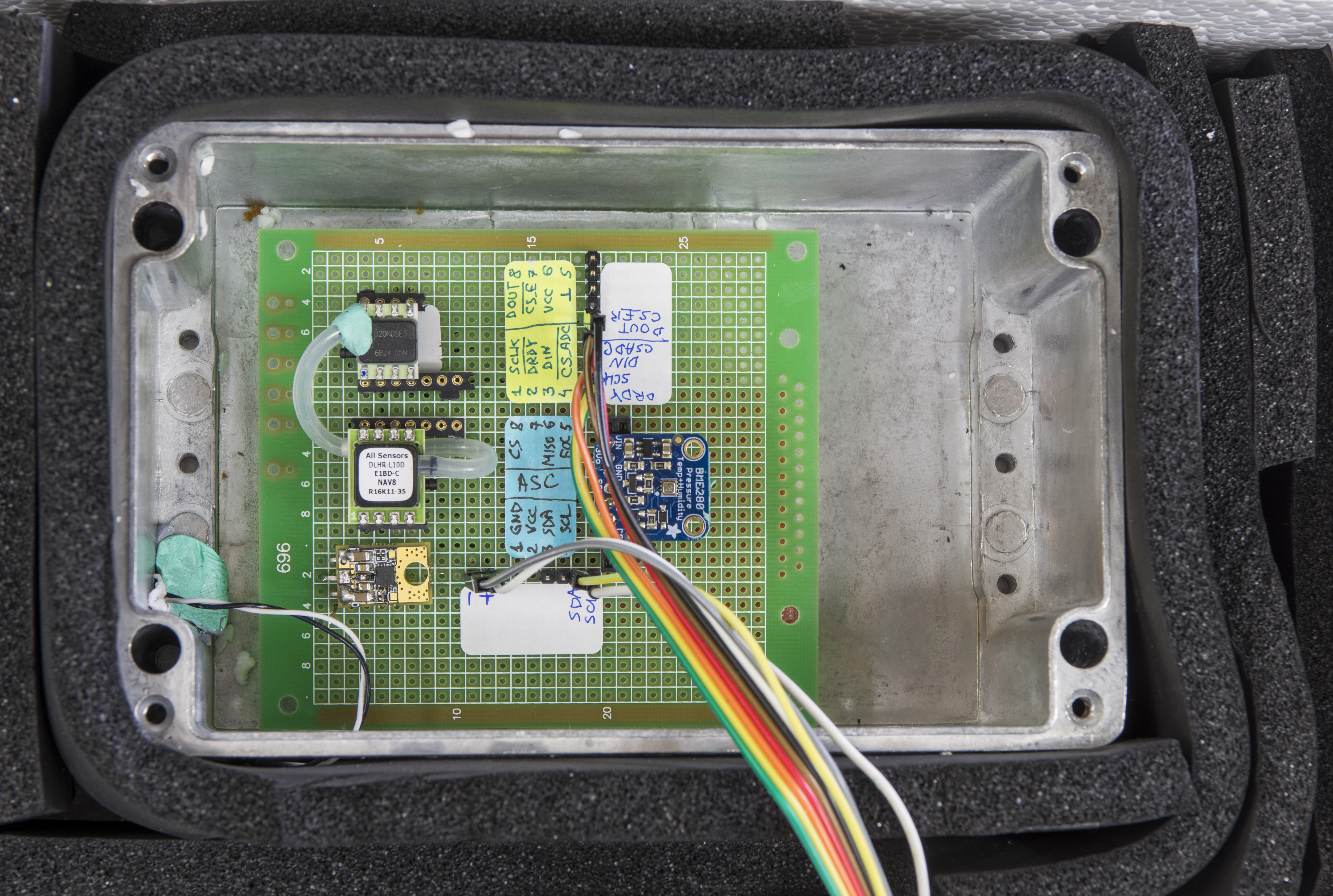
Image 38-39. Test setup, from left to right: Low-noise linear power supply, Allsensors DLHR sensor, Honeywell RSC sensor, BME280 (bottom).
Generic 40W 40×40mm TEC module with cooling heatsink attached to the bottom of the box, to allow active temperature control to desired temperature. To reduce impact and heat loss into ambient, whole box insulated with HVAC-grade foam and surrounded by styrofoam larger container. TEC setpoint, temperature control and power is maintained using Keithley 2510 TEC SMU.
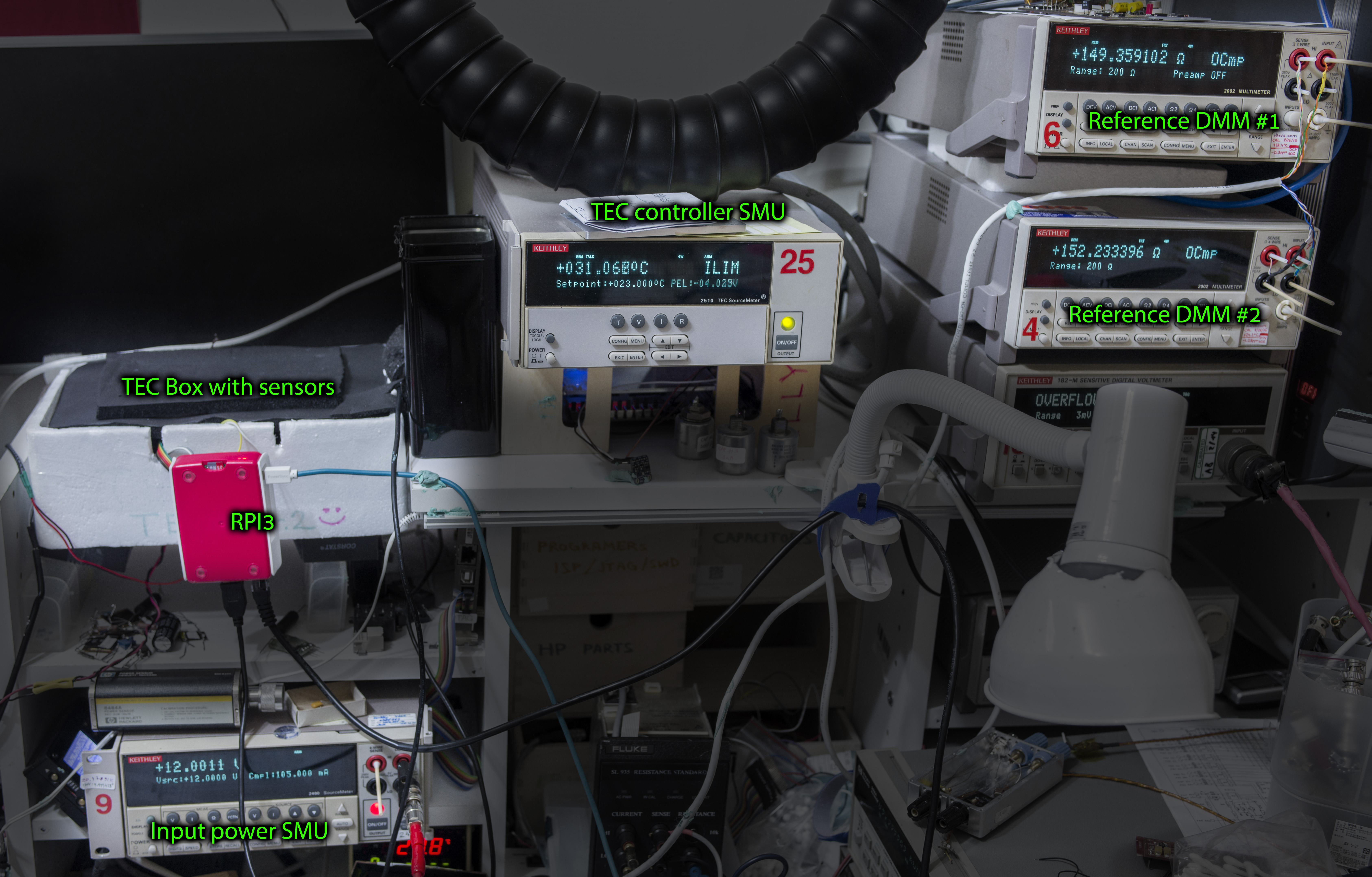
Image 40. Test equipment setup
All data collection from sensors and Keithley 2510 controlled by same Python application. Physical interface to Keithley is GPIB, with linux-gpib library used as software framework to Python. xDevs.com guides covering setup of Raspberry Pi Linux with both popular NI GPIB-USB-HS and Agilent 82357B already available online.
Sensor data samples in timed sequence, together with box temperature, which is read directly from Keithley 2510. Each 100 samples (equals about 2 minutes of time) setpoint temperature increased by +0.1 °C. After reaching +47.0 °C some soak time held, following ramp down sequence with same speed executed to bring box temperature down to initial near temperature. This allow to also confirm to get data in both directions while heating or cooling sensor under test.
Temperature / power supply dependency test
First performance indicator would be running same amount of samples and calculating Standard deviation for each sensor dataset. Lower SD meaning better resolution capability of sensor and less noisy readings. In other words SD is a quantification of uncertainty in collected measurement data.
| Device under test | Input signal | Setting | Scope | Histogram | Std.Dev, inH2O | Median value, inH2O |
|---|---|---|---|---|---|---|
| ASC DLHR-L10D | Zero, open ports | Fixed period, AVG8, 1000 samples | 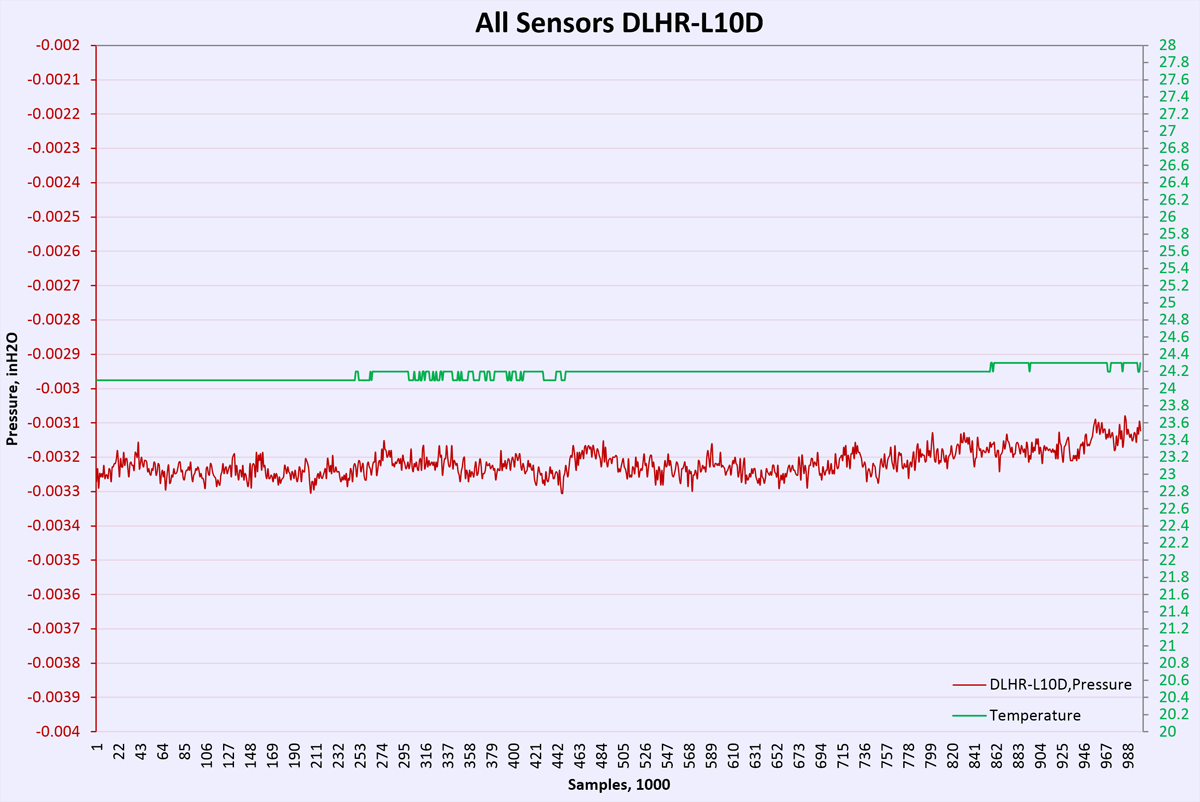 |
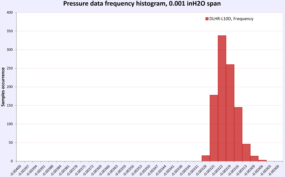 |
3.7939E-5 | -0.00322 |
| ASC DLHR-L02D | Zero, open ports | Fixed period, AVG8, 1000 samples | 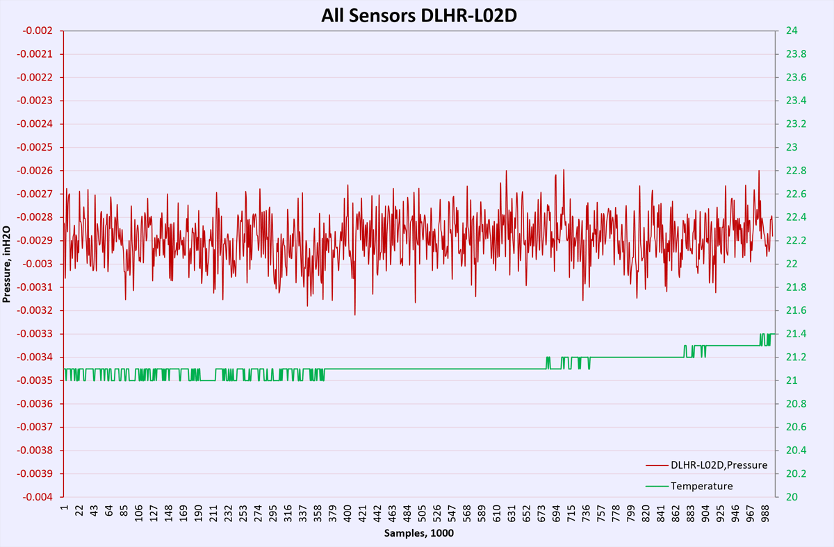 |
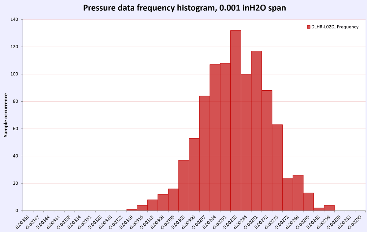 |
9.9588E-5 | -0.00289 |
| ASC DLHR-L01D | Zero, open ports | Fixed period, AVG8, 1000 samples |  |
 |
9.4646E-5 | 0.019497 |
| HW RSC020 | Zero, open ports | Fixed period, 20SPS, AVG8, 1000 samples | 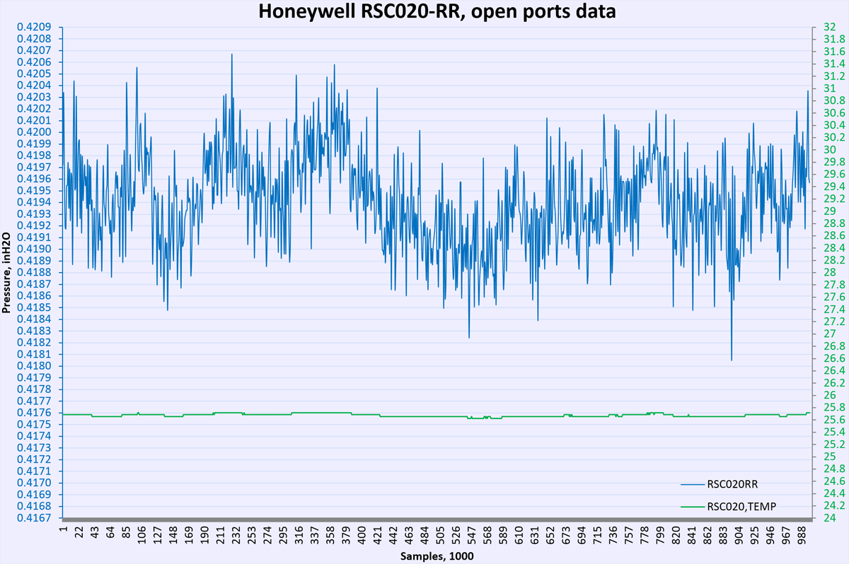 |
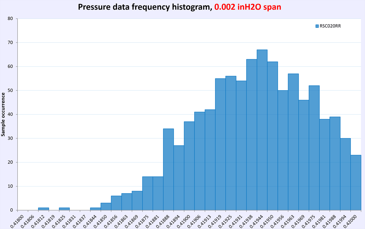 |
39.4183E-5 | 0.4194 |
| HW RSC002 | Zero, open ports | Fixed period, 20SPS, AVG8, 1000 samples | 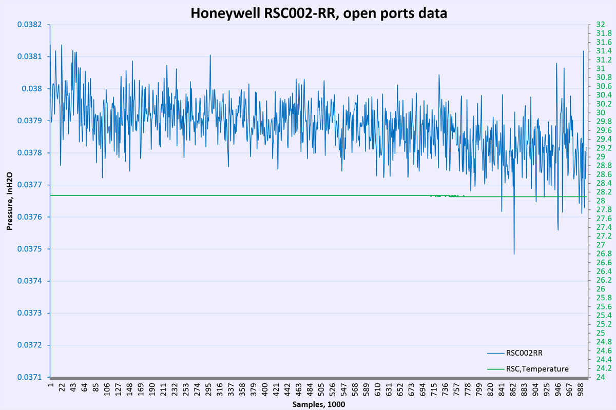 |
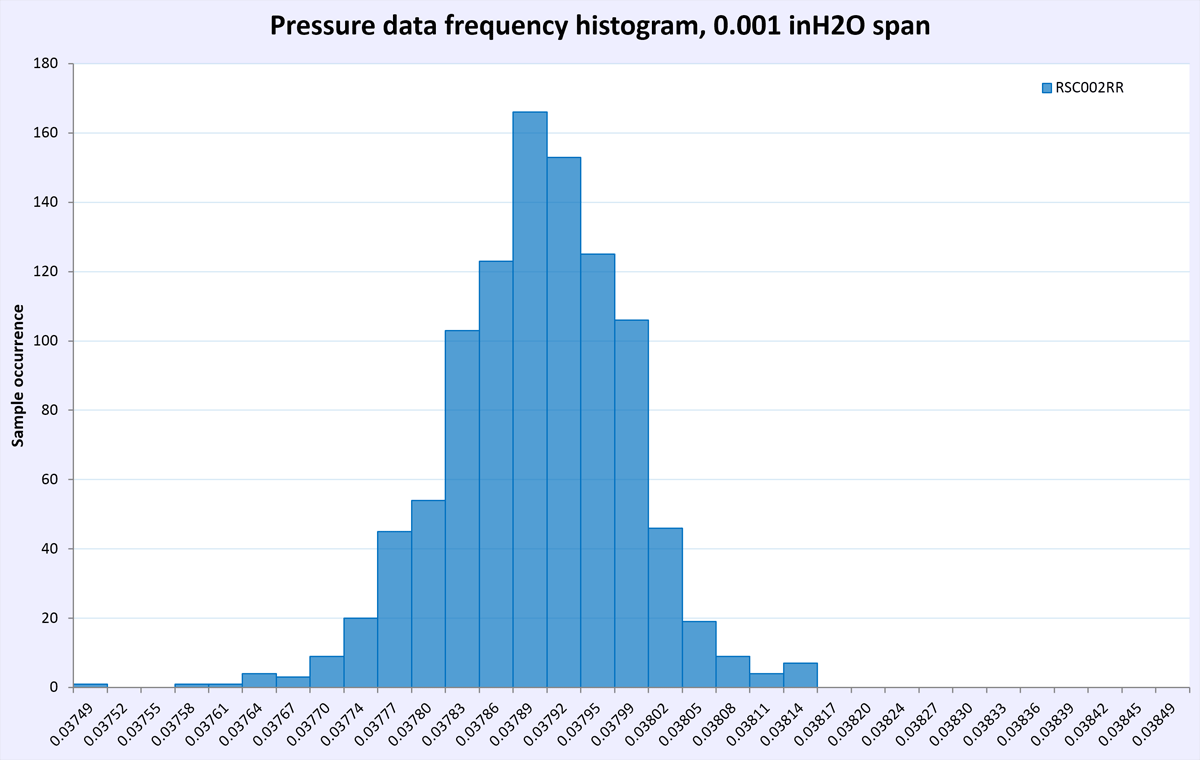 |
8.23824E-5 | 0.03789 |
Table 12: Zero short noise test results
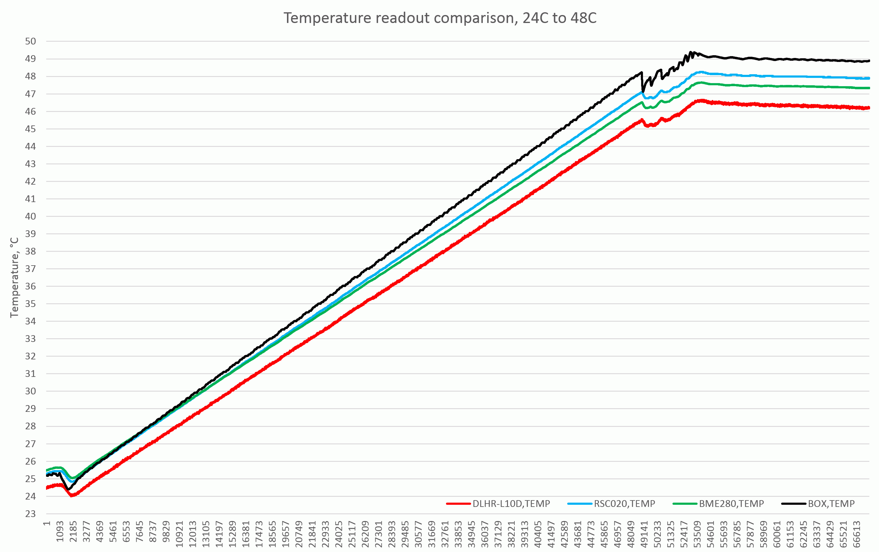
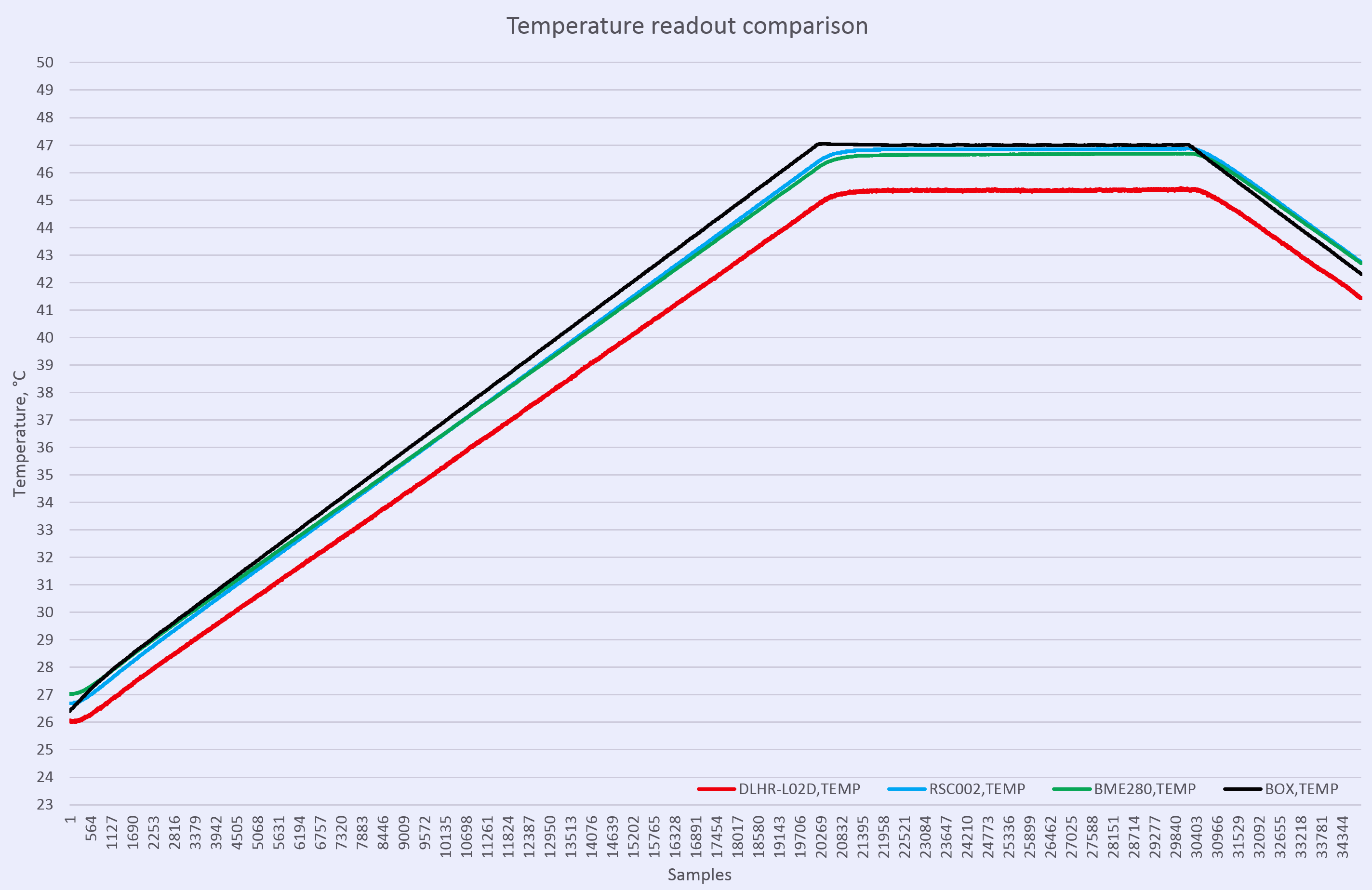
Temperature sensor linearity test can be done using TEC chamber fairly easy
 |
 |
 |
|
| Test temperature span | +26.0 °C … +47.0 °C | ||
Table 13: Temperature test plots
Offsets include total thermal chamber errors and sensor readout. There is no direct thermal coupling between reference RTD element and DUT’s, so larger values can be expected. What we looking for is linear and predictable temperature change, following airbath temperature raise (black line).
| Item | DLHR-L10D | DLHR-L02D | DLHR-L01D | RSC020RR | RSC002RR |
|---|---|---|---|---|---|
| +27 °C offset | -0.9 °C | -0.3 °C | -0.2 °C | 0.0 °C | -0.1 °C |
| +35 °C offset | -1.8 °C | -1.7 °C | -1.3 °C | -0.6 °C | -0.3 °C |
| +45 °C offset | -2.7 °C | -1.7 °C | -1.9 °C | -0.9 °C | -0.4 °C |
Table 14: Sensor results
Calibration test
In this test Fluke 719 calibrator will source known pressure into sensors and their output digital values will be recorded same time to compare calibration results. Second port of both sensors is open to atmosphere, converting differential sensor into simplified gauge.
| Reference input | Used sensors | Fluke 719 reading | ASC sensor | RSC sensor |
|---|---|---|---|---|
| -1.00 inH2O | DLHR-L01D + RSC002 | -1.00 inH2O | -1.008 (0.8%) | -0.938 (-6.2%) |
| -0.50 inH2O | DLHR-L01D + RSC002 | -0.50 inH2O | -0.4994 (-0.12%) | -0.474 (-5.2%) |
| -0.25 inH2O | DLHR-L01D + RSC002 | -0.25 inH2O | -0.2496 (-0.16%) | -0.242 (-3.2%) |
| 0.00 inH2O | DLHR-L01D + RSC002 | 0.00 inH2O | 0.004 | 0.002 |
| +0.25 inH2O | DLHR-L01D + RSC002 | +0.25 inH2O | 0.2561 (2.44%) | 0.247 (-1.2%) |
| +0.50 inH2O | DLHR-L01D + RSC002 | +0.50 inH2O | 0.5077 (1.54%) | 0.468 (-6.4%) |
| +1.00 inH2O | DLHR-L01D + RSC002 | +1.00 inH2O | 1.009 (0.9%) | 0.927 (-7.3%) |
Table 15: DHLR-L01D + RSC002 Comparison results with Fluke 719 30G calibrator output
Large offset was read from Honeywell RSC sensor. Additional calibration and compensation math may be required to provide better calibration results, so these results obviously need further investigation. Repeated test shown same numbers, so data provided here as is. Fluke 719 30G not the best tool to source low pressure levels below 5 inH2O either.
| Reference input | Used sensors | Fluke 719 reading | ASC sensor | RSC sensor |
|---|---|---|---|---|
| -2.00 inH2O | DLHR-L02D + RSC002 | -2.00 inH2O | -1.996 (-0.2%) | -1.869 (-6.5%) |
| -1.00 inH2O | DLHR-L02D + RSC002 | -1.00 inH2O | -1.001 (0.1%) | -0.932 (-6.8%) |
| -0.50 inH2O | DLHR-L02D + RSC002 | -0.50 inH2O | -0.507 (1.4%) | -0.467 (-6.6%) |
| 0.00 inH2O | DLHR-L02D + RSC002 | 0.00 inH2O | 0.001 | 0.008 |
| +0.50 inH2O | DLHR-L02D + RSC002 | +0.50 inH2O | 0.503 (0.6%) | 0.465 (-7%) |
| +1.00 inH2O | DLHR-L02D + RSC002 | +1.00 inH2O | 1.006 (0.6%) | 0.927 (-7.3%) |
| +2.00 inH2O | DLHR-L02D + RSC002 | +2.00 inH2O | 2.005 (0.25%) | 1.861 (-6.95%) |
Table 16: DHLR-L02D + RSC002 Comparison results with Fluke 719 30G calibrator output
Similar offset around 7% was detected from Honeywell RSC002 sensor as well. Code to interface sensor was reused, with correction for different pressure range. ASC sensor data was below 1.5%.
| Reference input | Used sensors | Fluke 719 reading | ASC sensor | RSC sensor |
|---|---|---|---|---|
| -20.00 inH2O | DLHR-L10D + RSC020 | -20.00 inH2O | N/A | -18.979 (-5.1%) |
| -15.00 inH2O | DLHR-L10D + RSC020 | -15.00 inH2O | N/A | -14.226 (-5.1%) |
| -12.00 inH2O | DLHR-L10D + RSC020 | -12.00 inH2O | -12.005 (0.04%) | -11.400 (-5%) |
| -10.00 inH2O | DLHR-L10D + RSC020 | -10.00 inH2O | -10.012 (-0.12%) | -9.531 (-4.69%) |
| -8.00 inH2O | DLHR-L10D + RSC020 | -8.00 inH2O | -8.017 (0.21%) | -7.614 (-4.82%) |
| -6.00 inH2O | DLHR-L10D + RSC020 | -6.00 inH2O | -6.018 (0.3%) | -5.688 (-5.2%) |
| -4.00 inH2O | DLHR-L10D + RSC020 | -4.00 inH2O | -4.004 (0.1%) | -3.793 (-5.17%) |
| -2.00 inH2O | DLHR-L10D + RSC020 | -2.00 inH2O | -2.015 (0.75%) | -1.902 (-4.9%) |
| -1.00 inH2O | DLHR-L10D + RSC020 | -1.00 inH2O | -1.007 (0.7%) | -0.944 (-5.6%) |
| 0.00 inH2O | DLHR-L10D + RSC020 | 0.00 inH2O | -0.02 | -0.008 () |
| +1.00 inH2O | DLHR-L10D + RSC020 | +1.00 inH2O | 1.010 (1%) | 0.958 (-4.2%) |
| +2.00 inH2O | DLHR-L10D + RSC020 | +2.00 inH2O | 2.002 (0.1%) | 1.904 (-4.8%) |
| +4.00 inH2O | DLHR-L10D + RSC020 | +4.00 inH2O | 3.997 (-0.075%) | 3.805 (-4.9%) |
| +6.00 inH2O | DLHR-L10D + RSC020 | +6.00 inH2O | 6.003 (0.05%) | 5.705 (-4.9%) |
| +8.00 inH2O | DLHR-L10D + RSC020 | +8.00 inH2O | 7.997 (-0.037%) | 7.586 (-5.2%) |
| +10.00 inH2O | DLHR-L10D + RSC020 | +10.00 inH2O | 9.998 (-0.02%) | 9.483 (-5.17%) |
| +12.00 inH2O | DLHR-L10D + RSC020 | +12.00 inH2O | 11.965 (-0.29%) | 11.381 (-5.15%) |
| +15.00 inH2O | DLHR-L10D + RSC020 | +15.00 inH2O | N/A | 14.221 (-5.2%) |
| +20.00 inH2O | DLHR-L10D + RSC020 | +20.00 inH2O | N/A | 18.964 (-5.18%) |
Table 17: DHLR-L10D + RSC020 Comparison results with Fluke 719 30G calibrator output
Here apparent error of RSC output was visible and very high, requiring addition correction for 5% offset. Good indication that higher resolution on it’s own does not guarantee better accuracy of the system.
Given unknown calibration or use history of Fluke 719 used in this test, obtained results are good, mostly well under 1% for All Sensors DLHR sensor. Thanks to onboard DSP, which handled all calibration and internal data correction, using DLHR-LxxD sensor was very easy and straight-forward.
Honeywell RSC however had extra offset, which need to be manually corrected. Compensation for RSC sensor was performed according to datasheet listed math and stored EEPROM data.
As side note, Fluke 719 30G pressure range is not optimal to perform accurate calibration/test, so take data presented as is.
Summary & Conclusion
This article brought us example of what modern digital electronics can do together with proven technology. Years ago you needed significant amount of knowledge to implement pressure measurement into the system, starting from sensor design, low-noise and stable front end for it, measurement system and compensation methods. Easy to imagine expensive large assembly with tens and tens of components on it just to get all that to work.
Today however even students without any practical electronics design background can get parts, connected them to popular platform like linux-based Raspberry Pi or Arduino and get first pressure measurements in matter of hours, not weeks. And that is already calibrated and compensated value, ready to be used for further processing in application. Teardown of sensors also help to learn a little how such things work and how they are designed.
Such temperature-compensated silicon pressure sensors have reachable price and package to be used widely. Also their accuracy and digital compensation making them attractive in wide variety of precision sensing projects. Flow metering, liquids level, process monitoring, research, optical power detection and many more. Looking forward for future sensors with integrated buffers, 50/60Hz rejection, and overall system calibration can further reduce pressure systems complexity and cost.
If you like this study, please let us know for further experiments and ideas. Any corrections or suggestions are welcome!
Projects like this are born from passion and a desire to share how things work. Education is the foundation of a healthy society - especially important in today's volatile world. xDevs began as a personal project notepad in Kherson, Ukraine back in 2008 and has grown with support of passionate readers just like you. There are no (and never will be) any ads, sponsors or shareholders behind xDevs.com, just a commitment to inspire and help learning. If you are in a position to help others like us, please consider supporting xDevs.com’s home-country Ukraine in its defense of freedom to speak, freedom to live in peace and freedom to choose their way. You can use official site to support Ukraine – United24 or Help99. Every cent counts.
Modified: Jan. 1, 2024, 8:33 p.m.
References
- Python official site
- All Sensors DLHR Series Pressure Sensor page
- ASC DLHR datasheet
- All Sensors white and application notes
- Honeywell RSC series pressure sensors
- Honeywell RSC datasheet
- Fluke 719 30G pressure calibrator page
- Raspberry Pi foundation official website
- www.raspberrypi-spy.co.uk : Raspberry Pi B+ Pinout
- Linear : LT3042 low-noise LDO
- Keithley 2510 TEC SMU controller
- Setting up and using Agilent 82357B GPIB USB pod in RPi Linux
- Texas Instruments ADS1220 ADC page
- xDevs.com Pressure Demo application repository
- Understanding Smart Sensors, Third Edition by Randy Frank