• Introduction
• Disclaimer
• Design and compensation process
• xDevs TCkit : TCR plotting and analytics script tests
• Conclusion

Introduction and motivation

This short article is provided to encourage and motivate people to build and temperature compensate their own resistor references. Why would you bother with the temperature coefficient (TCR for short) in the first place, if you can simply measure the temperature and calculate the correction for it? The answer to it is the convenience when dealing with your resistance reference, very useful for experiments such as transfer between two meters. For practical and useful values three nominal values were selected for this build.

Disclaimer

Redistribution and use of this article, any part of it or any images or files referenced in it, in source and binary forms, with or without modification, are permitted provided that the following conditions are met:

• Redistributions of article must retain the above copyright notice, this list of conditions, link to this page (https://xdevs.com/article/3rref_tcrt/) and the following disclaimer.
• Redistributions of files in binary form must reproduce the above copyright notice, this list of conditions, link to this page (https://xdevs.com/article/3rref_tcrt/), and the following disclaimer in the documentation and/or other materials provided with the distribution, for example Readme file.

All information posted here is hosted just for education purposes and provided AS IS. In no event shall the author, xDevs.com site, Vishay Precision Group or any other 3rd party be liable for any special, direct, indirect, or consequential damages or any damages whatsoever resulting from loss of use, data or profits, whether in an action of contract, negligence or other tortuous action, arising out of or in connection with the use or performance of information published here.

If you willing to contribute or add your experience regarding instrument repairs or provide extra information, you can do so following these simple instructions.

Design and compensation process

On the other hand the effort to compensate is rather low, all it takes is patience to wait for the temperature sweeps to complete, to pick up the results, calculate what to do next, modify the reference and measure again. You might end up overcompensating things, but that should not stop you from trimming until you are happy with the final result.

A few resistors came in handy to build another DIY resistance reference, namely 3x VPG VHP202 Y0024 with nominal values of 100 Ω, 1 kΩ and 10 kΩ.

All three resistors were mounted in a 120 × 80 × 51 mm³ Rose aluminum die cast box [1] connected to Stäubli PK4T binding posts. A TE GA10k31 thermistor was added and thermally attached to the common leads of the resistors.

The initial TCR of the resistors after assembly was measured in a temperature range between +18 … 28 °C using a home-brew thermal chamber based on a modified incubator with Arroyo 5305 TEC controller. A Solartron 7081 in “true ohms” mode, 7×9 was used to measure resistance, which takes about 6.4 seconds for each reading with resolution 7½ digits.

As Figure 1, 2 and 3 indicate a linear and negative temperature coefficient was found for all three specimen, which can be perfectly compensated using the TCR of some copper wire. The initial TCR numbers are listed in Table 1.

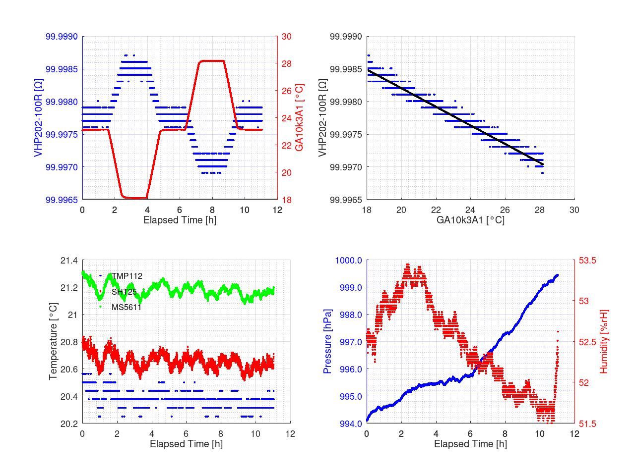
Figure 1: Initial temperature coefficient measurement of VHP202-100R

Same test repeated for 1000 Ω element output.

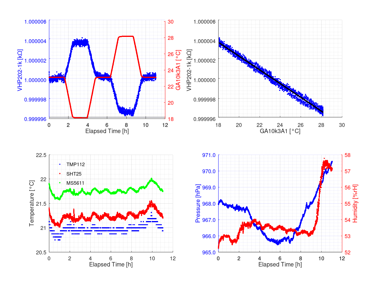
Figure 2: Initial temperature coefficient measurement of VHP202-1k

And finally 100 Ω output measurements:

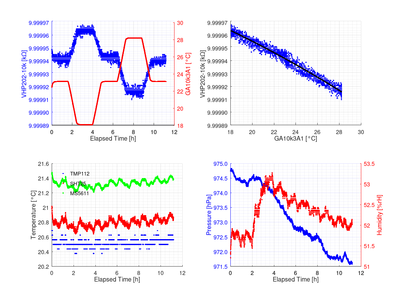
Figure 3: Initial temperature coefficient measurement of VHP202-100R

Based on these data samples it is easy to determine overall linear TCR in temperature range from +18 °C to +28 °C.

Resistor	Initial TCR
VHP202-100	-142.38 µΩ/K or -1.42 µΩ/Ω/K
VHP202-1k	-706.36 µΩ/K or -0.7 µΩ/Ω/K
VHP202-10k	-4.679 mΩ/K or -0.47 µΩ/Ω/K

Table 1: Measured initial TCR for each the outputs

These experimental results align well with VPG’s promised maximum TCR specifications ±2.5 µΩ/Ω/K for VHP202 series resistors. To get even better TCR without complexity of ovens and custom metalwork, we may want to have these resistors with added TCR compensation network. This trick is not new, but it’s rarely used in any production equipment because it takes some of time to test and perform for each resistive standard build. The wire used for compensation (so called verowire) has a diameter of 0.2 mm, a resistance of 0.875 Ω/m, while copper shows positive a TCR of α = 3930 µΩ/Ω/K and β = 0.6 µΩ/Ω/K. As β component is small it can be neglected for the calculations of the required wire length, though the solder joints have to be added on both ends to the total length.

Keep in mind that this simple method would only work for resistors that exhibit negative TCR (increasing temperature causes resistance to decrease). Copper wire adds positive component to overall TCR. To compensate positing TCR element one would need to use arrangement with array of elements.

A simple spreadsheet was used for calculations and the following lengths were estimated (VHP202-100R: 52 mm, VHP202-1k: 206 mm, VHP202-10k: 1377 mm). From here it is an easy task of using a ruler and to measure the appropriate length of the wire, which was then bifilar wound onto the resistor cases and secured with some adhesive.

Afterwards the TCR sweeps were repeated. Figure 4, 5 and 6 show the results of these sweeps.

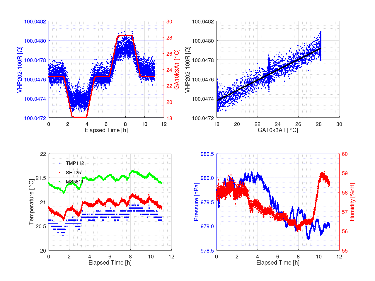
Figure 4: Temperature coefficient measurement of VHP202-100R after first TCR compensation

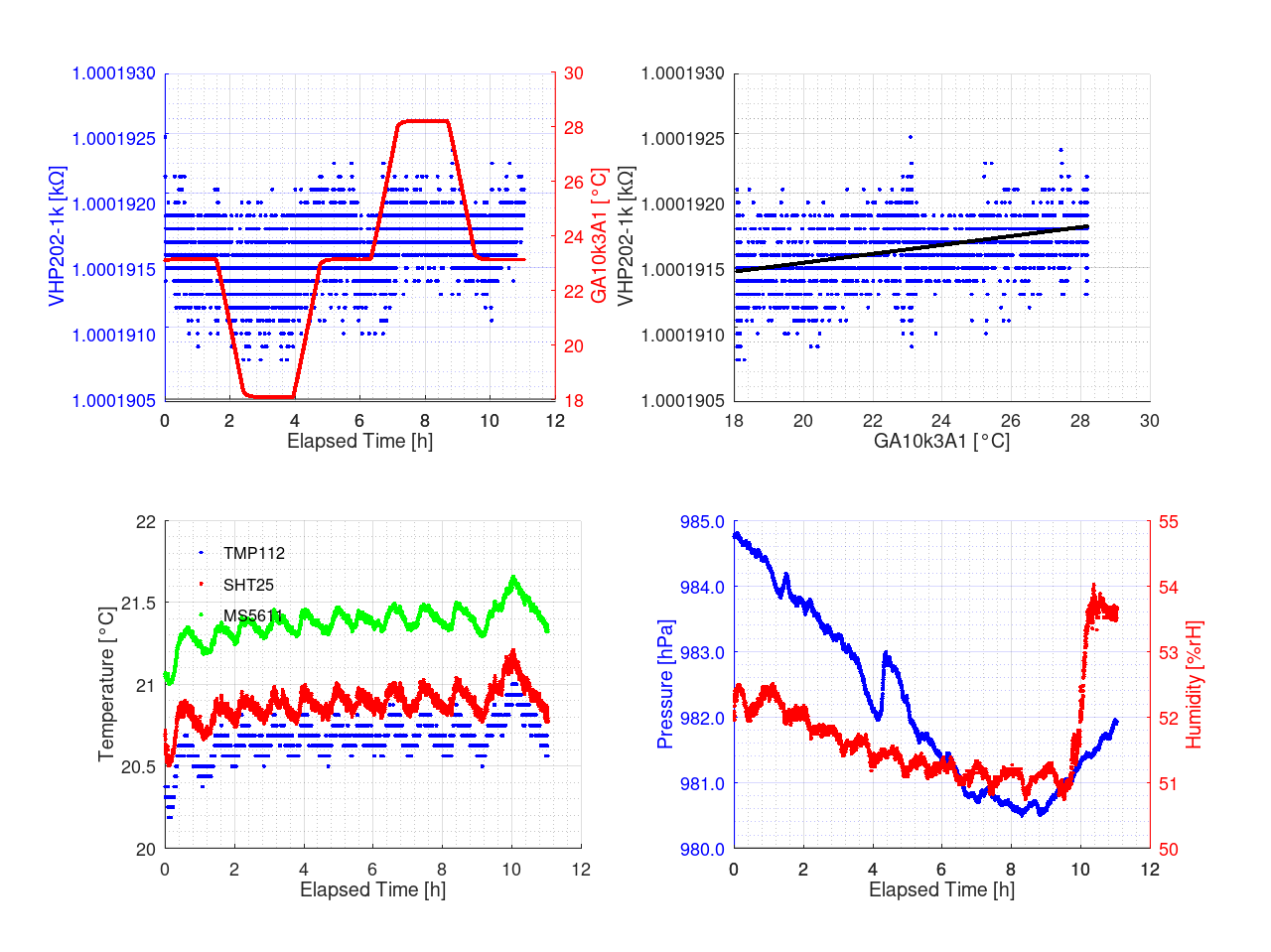
Figure 5: Temperature coefficient measurement of VHP202-1k after first TCR compensation

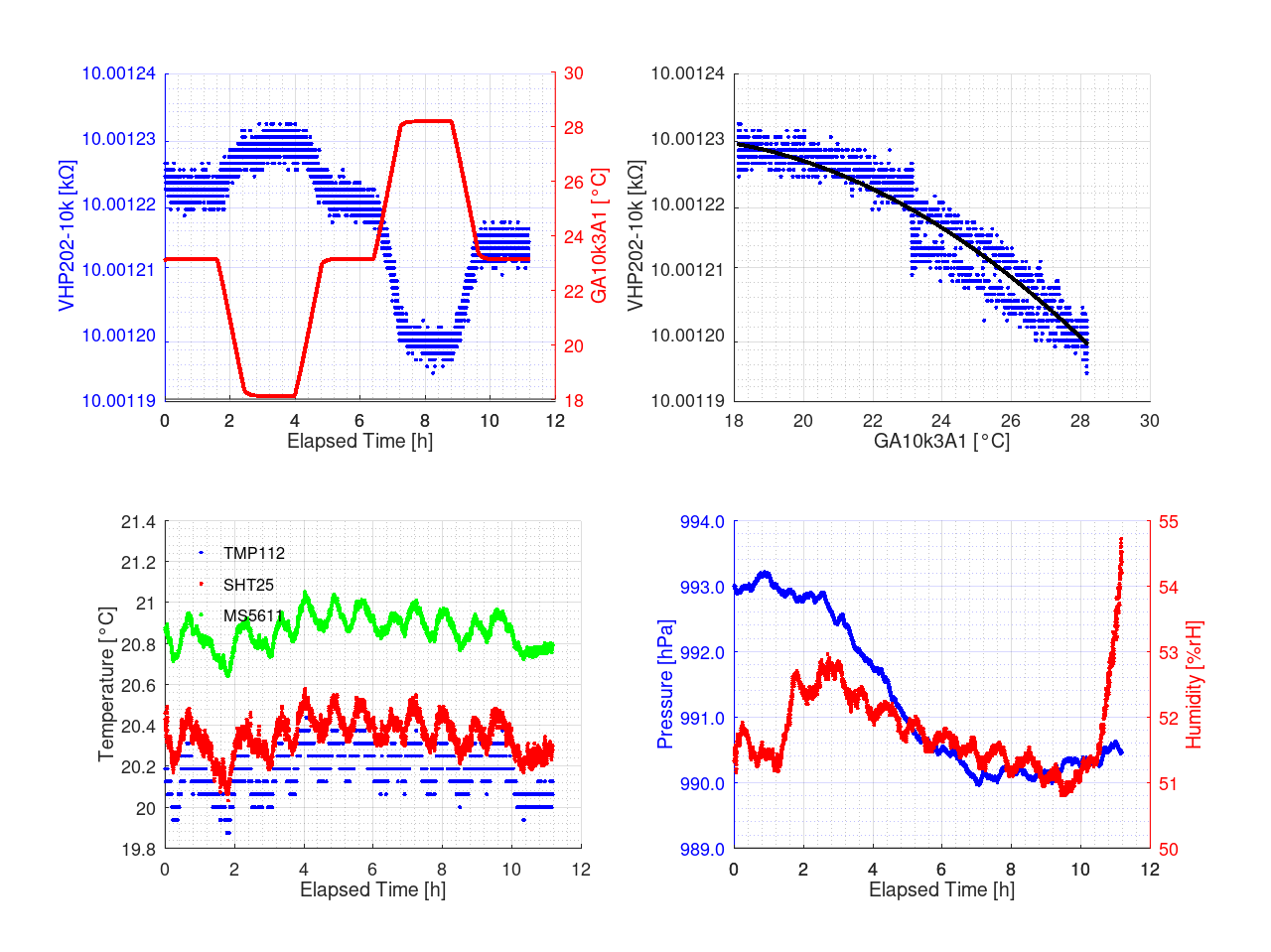
Figure 6: Temperature coefficient measurement of VHP202-10k after first TCR compensation

While VHP202-100R and VHP202-1k were overcompensated, something went obviously wrong for VHP202-10k, so the compensation and measurement was repeated for it, while the other two were trimmed to further improve TCR. Table 2 shows the related numbers for the TCR after the first compensation.

Resistor	TCR after compensation
VHP202-100	53.3 µΩ/K or 0.53 µΩ/Ω/K
VHP202-1k	33.9 µΩ/K or 0.034 µΩ/Ω/K
VHP202-10k	?

Table 2: T.C. after first compensation experiment

Figure 7, 8, 9 show the results. Again VHP202-10k didn’t work out well, hence the choice was made to reduce copper wire diameter and thus wire length. A 60 μm diameter enameled copper wire was used instead, which reduced the required wire length to below 200 mm.

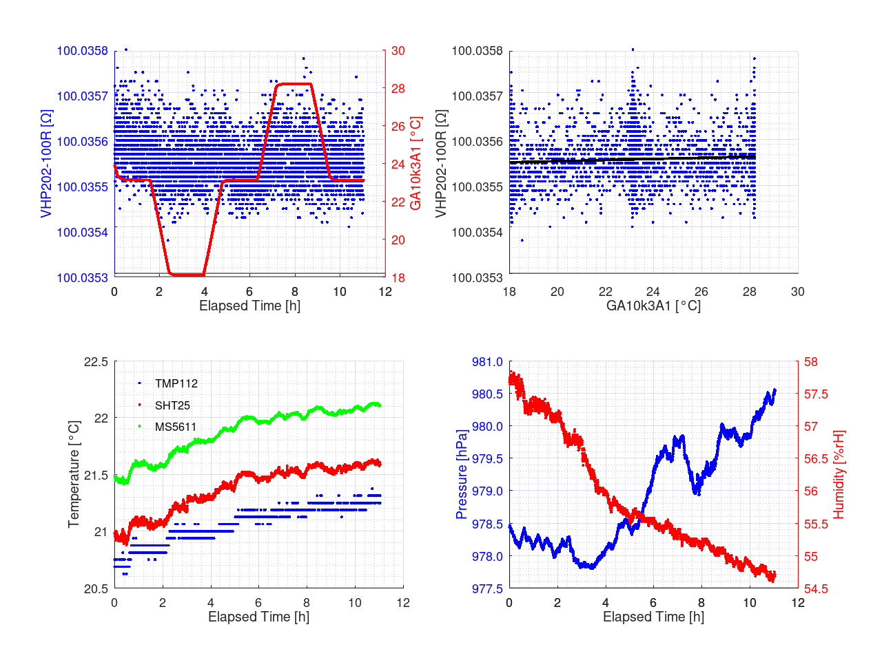
Figure 7: Temperature coefficient measurement of VHP202-100R after trimming

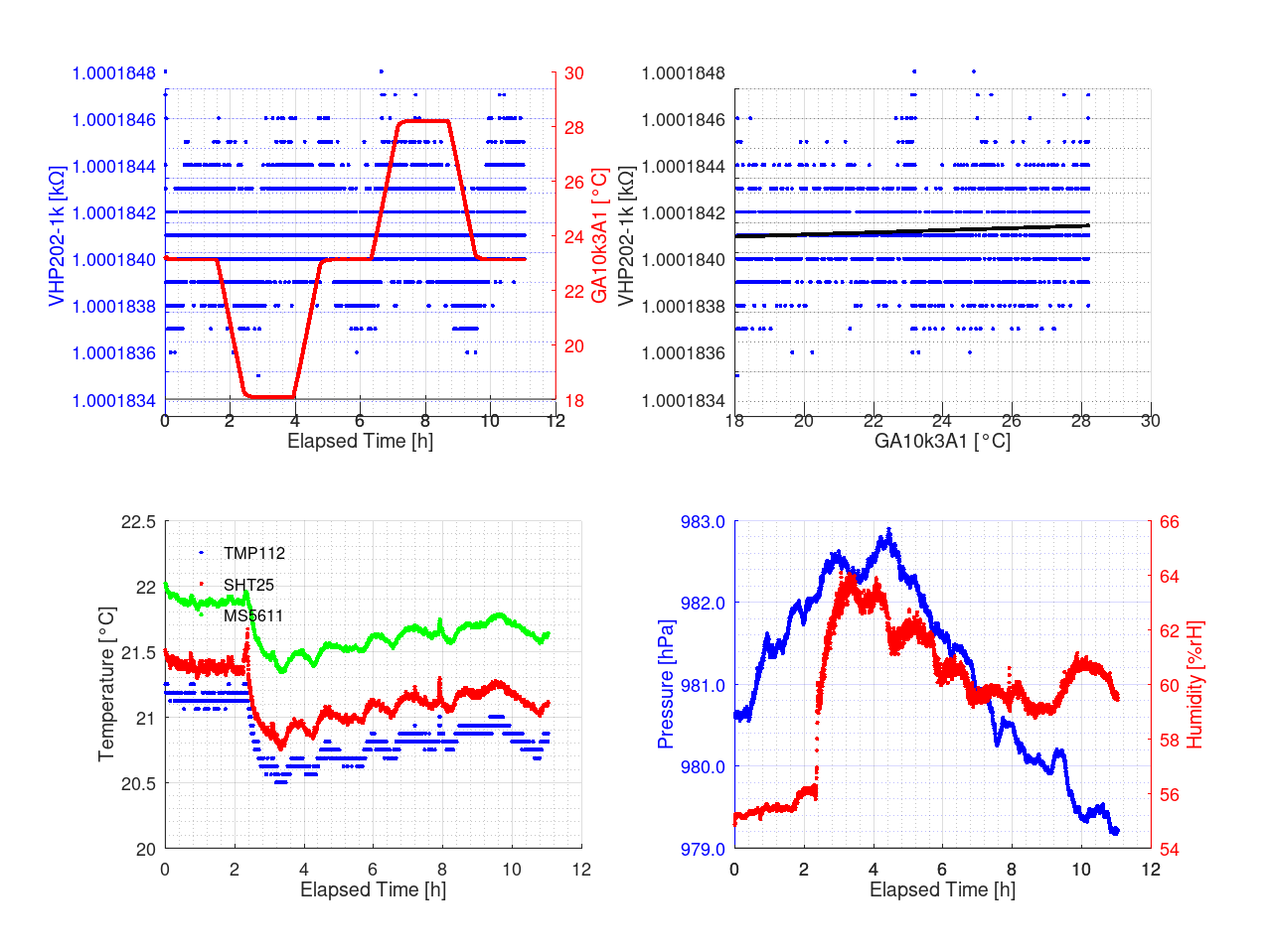
Figure 8: Temperature coefficient measurement of VHP202-1k after trimming

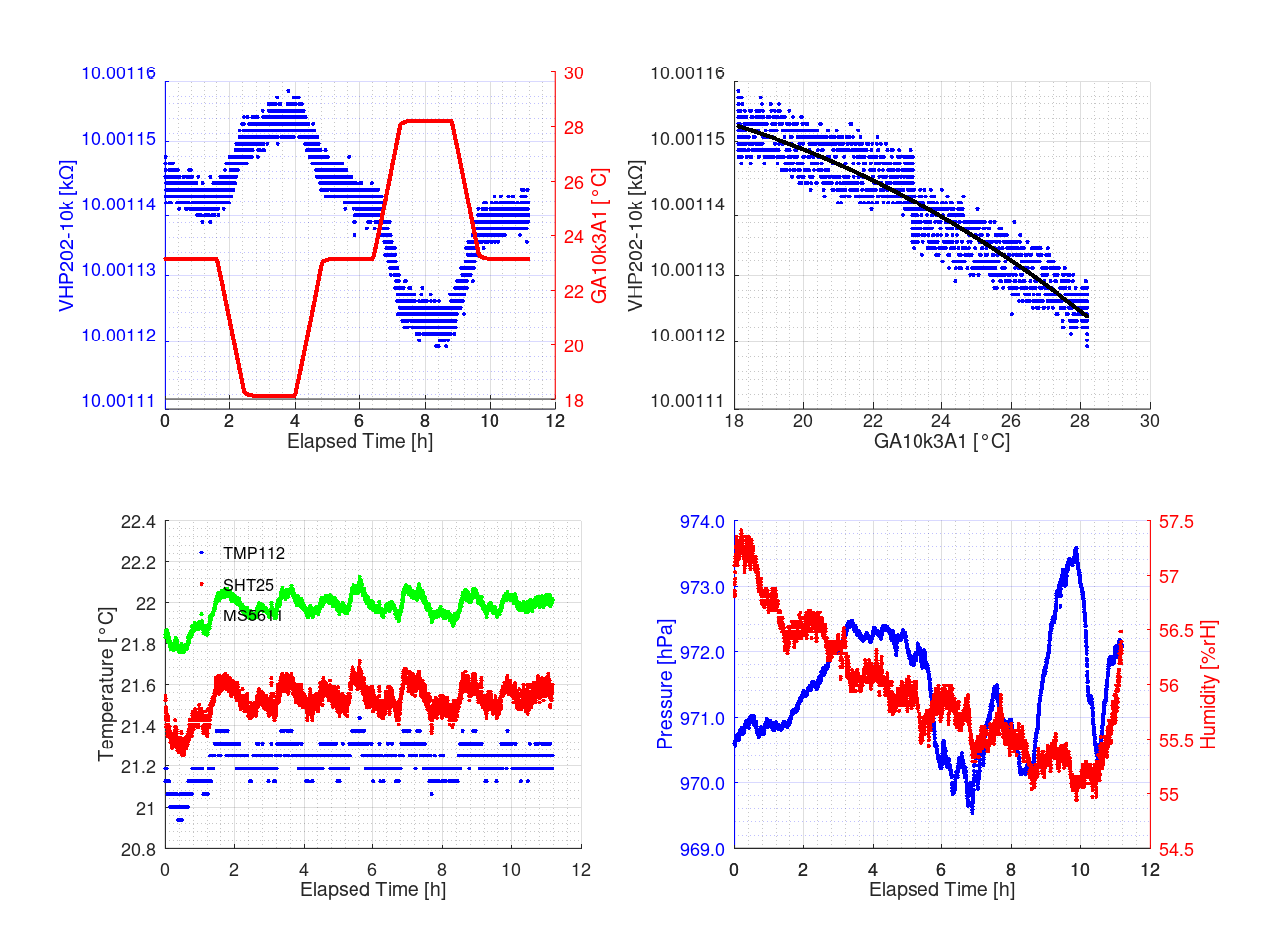
Figure 9: Temperature coefficient measurement of VHP202-10k after new TCR compensation

Figure 10 is the result of the temperature sweep after this modification. While slightly overcompensated a huge improvement is visible, but additional trimming was required and applied next.

This led to the conclusion, that the c.t.e. of the copper wire could have been the culprit. My personal conclusion from this experiment is to better use a wire diameter that ensures a small wire length such as <200 mm. While this is not a hard limit in any way, it’s what worked in this project and will be applied to the resistor used in [2] for verification.

Resistor	TCR after compensation
VHP202-100	1.24 µΩ/K or 0.0124 µΩ/Ω/K
VHP202-1k	4.64 µΩ/K or 0.00464 µΩ/Ω/K
VHP202-10k	368 µΩ/K or 0.0368 µΩ/Ω/K

Table 3: TCR after trimming

After a final trim VHP202-10k ended up with a TCR of 0.01 µΩ/Ω/K that is limited by the noise of the Solartron 7081 in the temperature range investigated, see Figure 11. The Solartron 7081 could have been set to 8×9 8½-digit mode, but then each reading sample would have taken 1 min 44 s in “true ohms” mode. A small humidity effect seems to show up in the measurement, but it’s unclear what was the source of the influence.

Table 4 shows the calculated TCR values in the more familiar 2-order polynomial form around 23 °C.

Resistor	TCR after final round of compensations
VHP202-100	αT23 = 0.013 µΩ/Ω/K , βT23 = -0.001 µΩ/Ω/K²
VHP202-1k	αT23 = 0.0043 µΩ/Ω/K , βT23 = 0.0015 µΩ/Ω/K²
VHP202-10k	αT23 = -0.0103 µΩ/Ω/K , βT23 = -0.0048 µΩ/Ω/K²

Table 4: Final αT23 and βT23 coefficients for the resistors

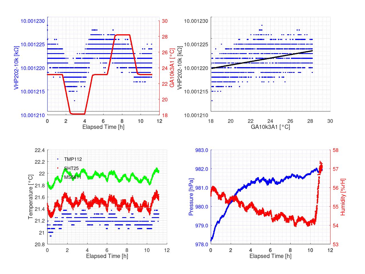
Figure 10: Temperature coefficient measurement of VHP202-10k after compensation with 60 μm enameled wire

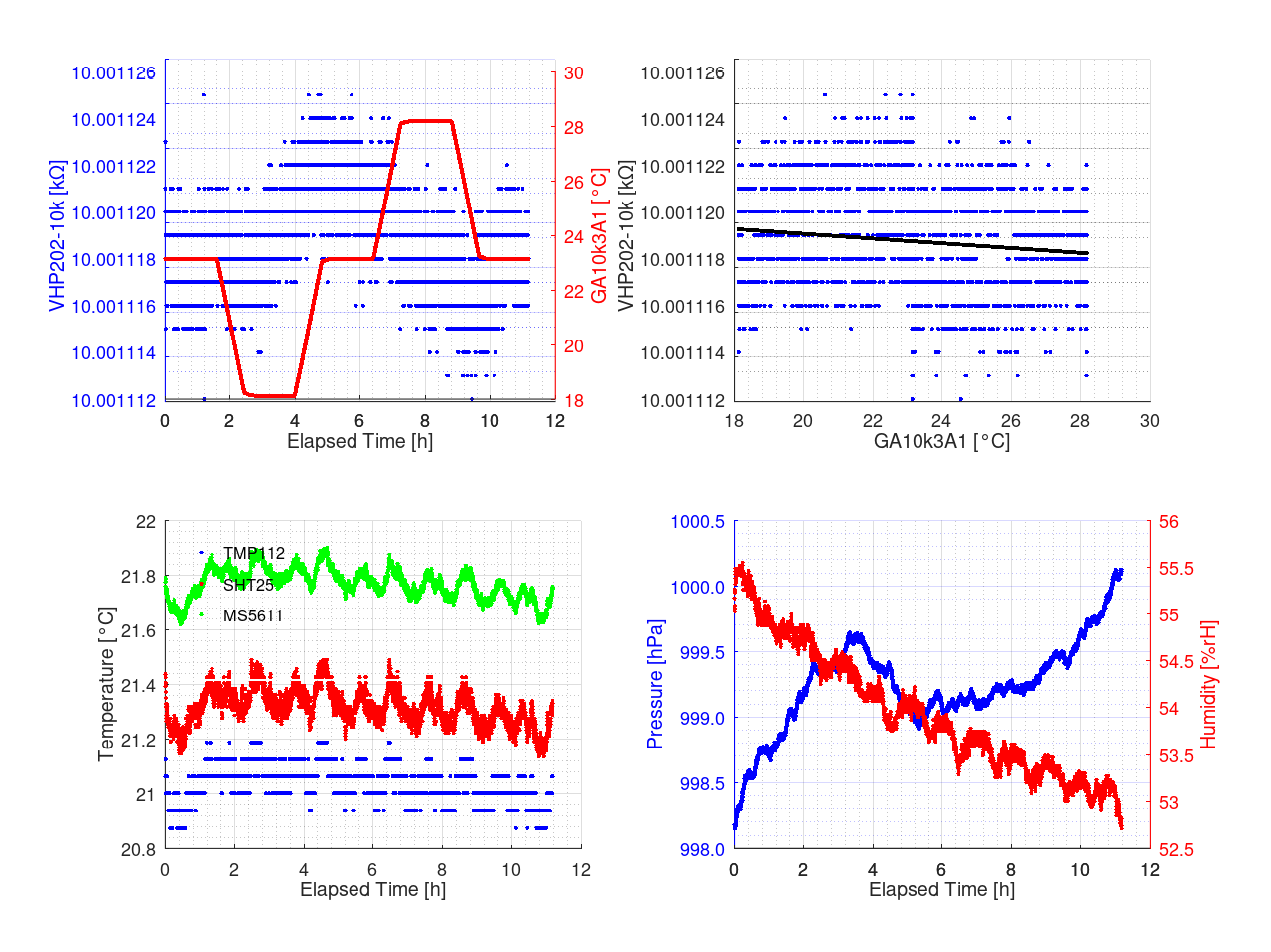
Figure 11: Temperature coefficient measurement of VHP202-10k after trimming

And finally, images (Figure 12 and 13) of the box were taken to present the build.

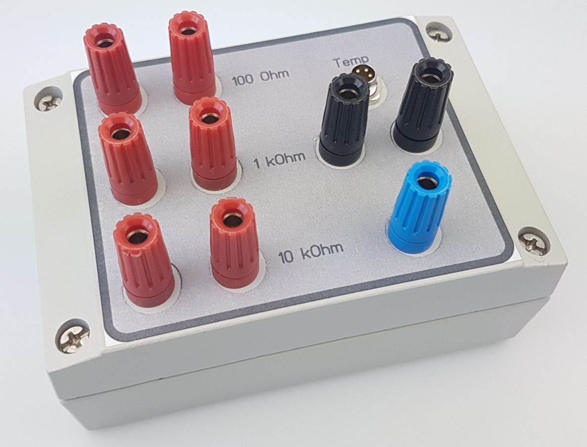
Figure 12: DIY triple resistor reference based on VHP202

Photographs demonstrate physical construction of the build. Sometimes few photographs can explain the topic better than two pages of text. Internal design is pretty simple and can be done even by modestly equipped lab.

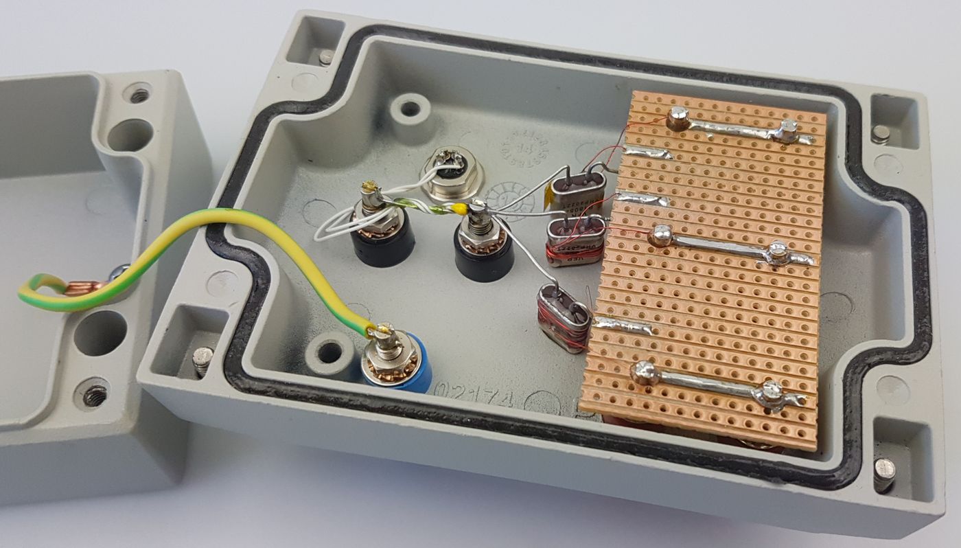
Figure 13: The guts of the DIY triple resistor reference based on VHP202

Coupling compensation copper wire to resistor body helps with better thermal coupling and mechanical rigidity of whole arrangement.

xDevs TCkit : TCR plotting and analytics script demo

Perhaps this article can be a good demonstration of the power and capabilities of open-source software and libraries for data processing and metrology experiments. Using such open tools number of members at xDevs developed and tested small script that is helping metrology studies. The codebase is currently available on github and tested with various data examples, even with multi-channel data acquired from the different DUTs in the same temperature chamber. Below are scripts and plots generated for this DIY 3-output box as a sample use case. Script is a bit messy but it can be a good template to work on.

xDevs.com TCkit Python3.9 script for plotting

This script takes CSV-file and generates PNG-files with plots. Script was tested with Python 3.9 and open libraries matplotlib 3.3.4, numpy 1.23.5 and scipy 1.10.0. Same CSV-files were used to both analysis above and here, to compare the algorithms and numbers.

xDevs.com analytics TCkit run with 100 Ω element output

CSV-file with TCR data, VPG 100 Ω element

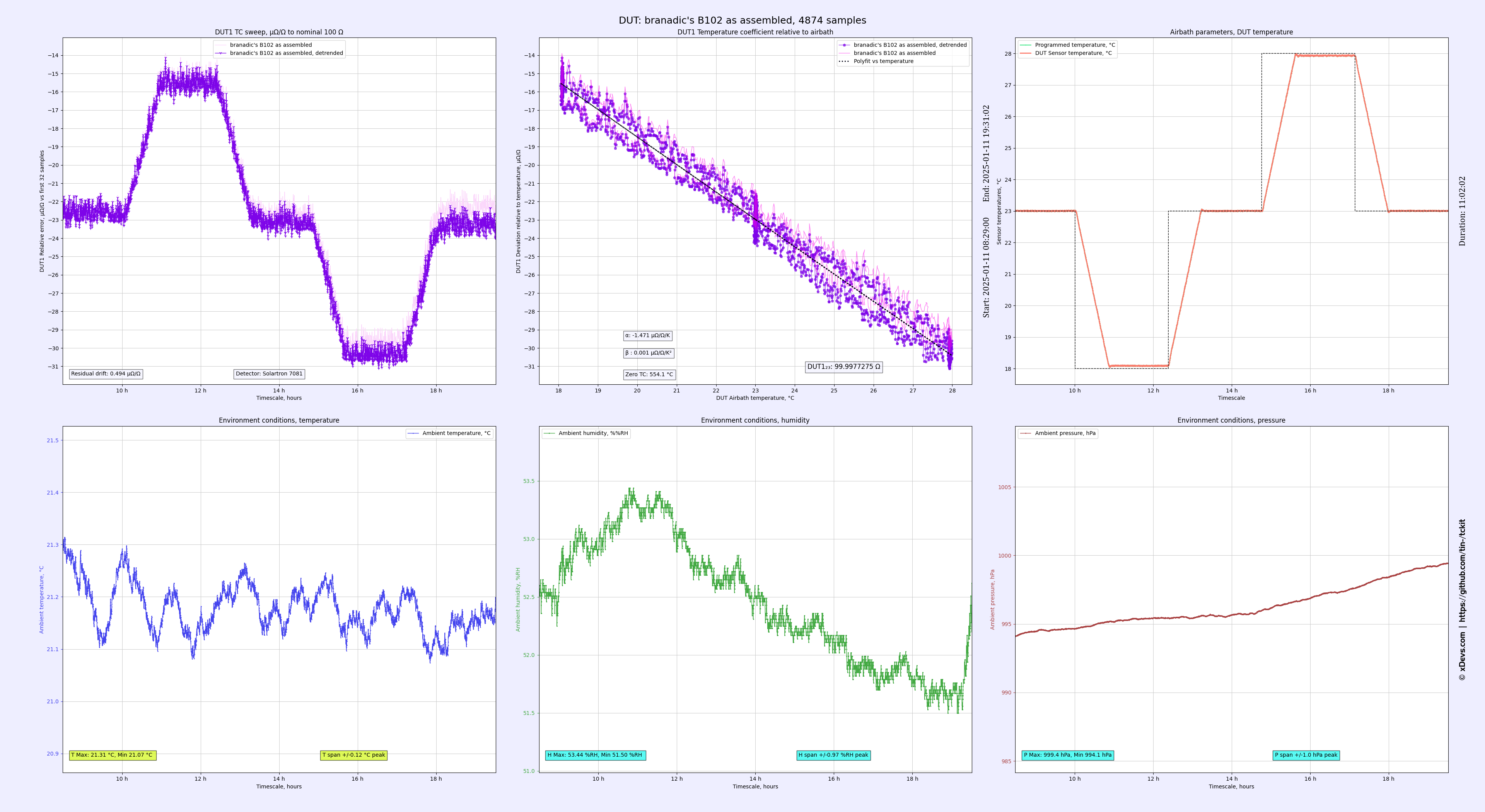
Figure 14: 100 Ω analytics as assembled

CSV-file with TCR data, VPG 100 Ω element

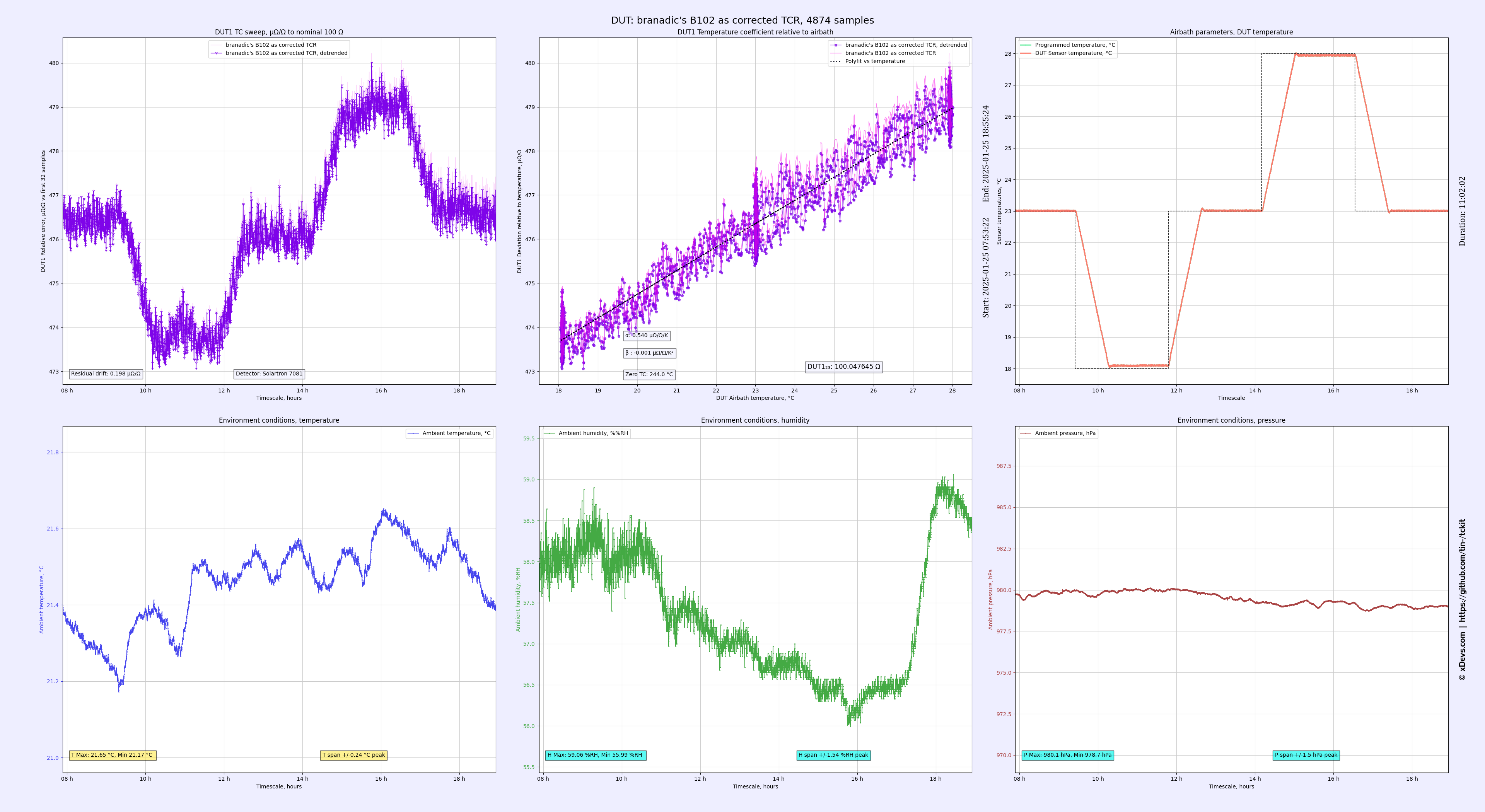
Figure 15: 100 Ω analytics after first TCR trim

CSV-file with TCR data, VPG 100 Ω element

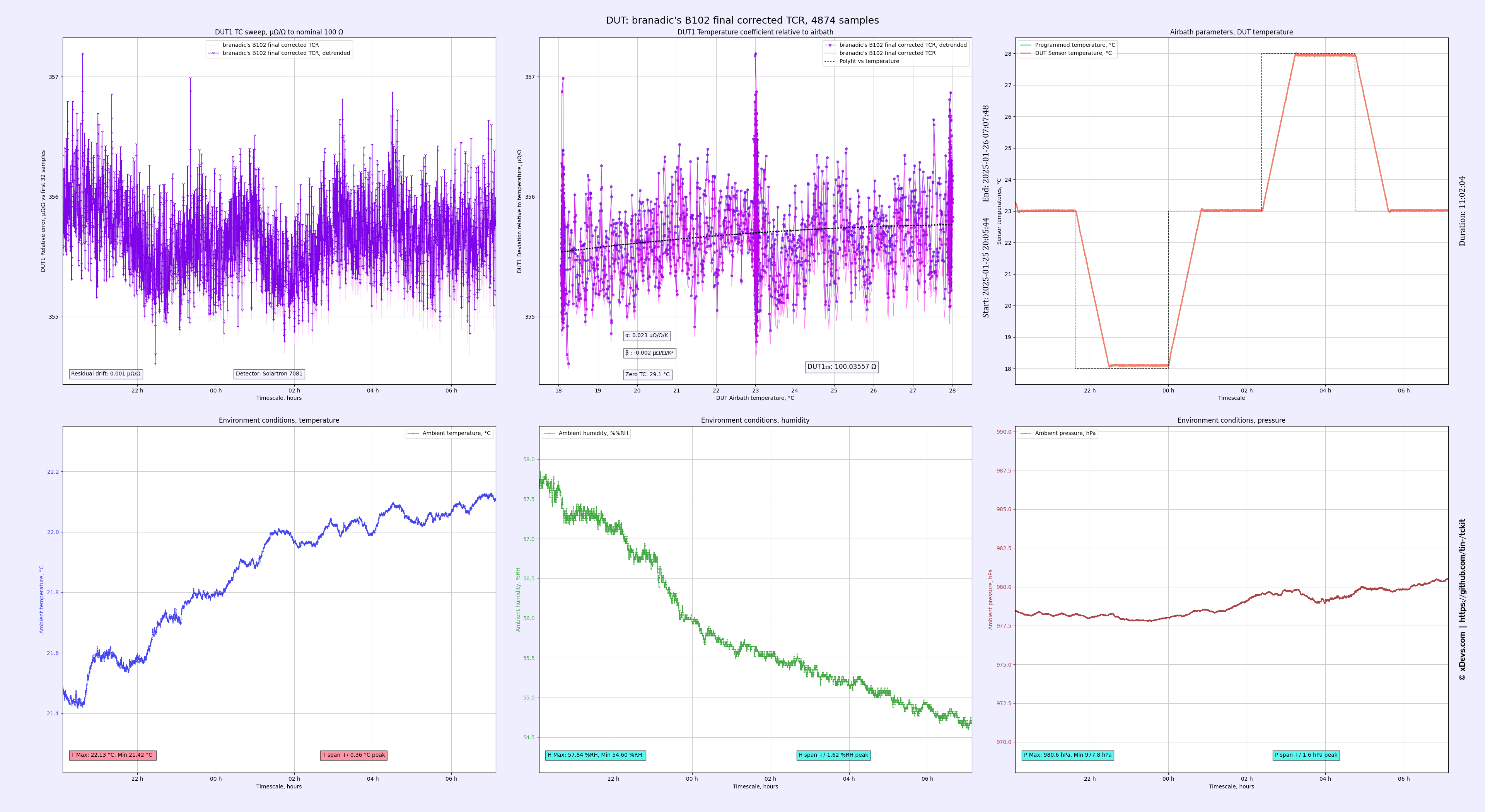
Figure 16: 100 Ω analytics final TCR trim

xDevs.com analytics TCkit run with 1 kΩ element output

CSV-file with TCR data, VPG 1 kΩ element

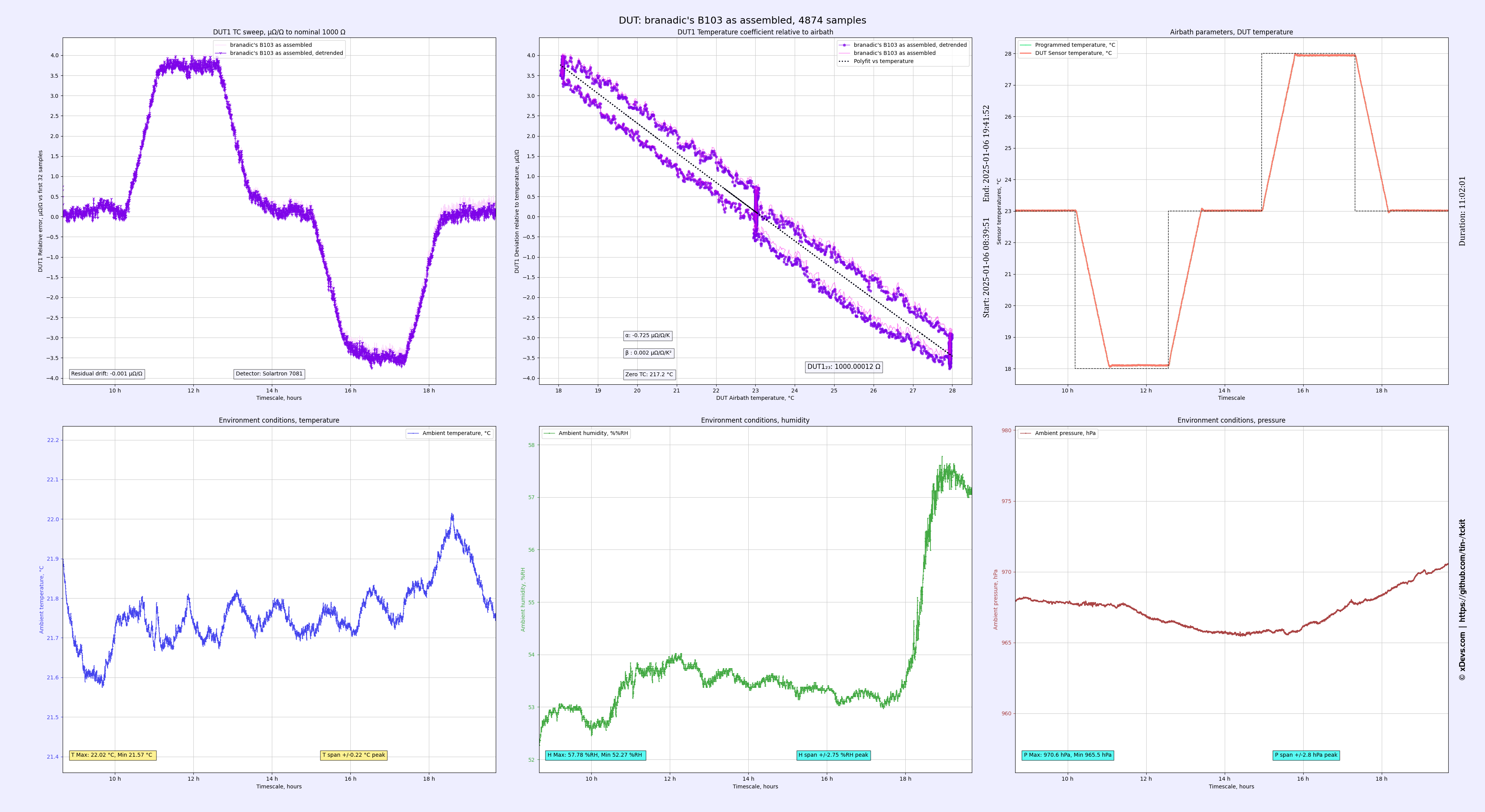
Figure 17: 1000 Ω analytics as assembled

CSV-file with TCR data, VPG 1 kΩ element

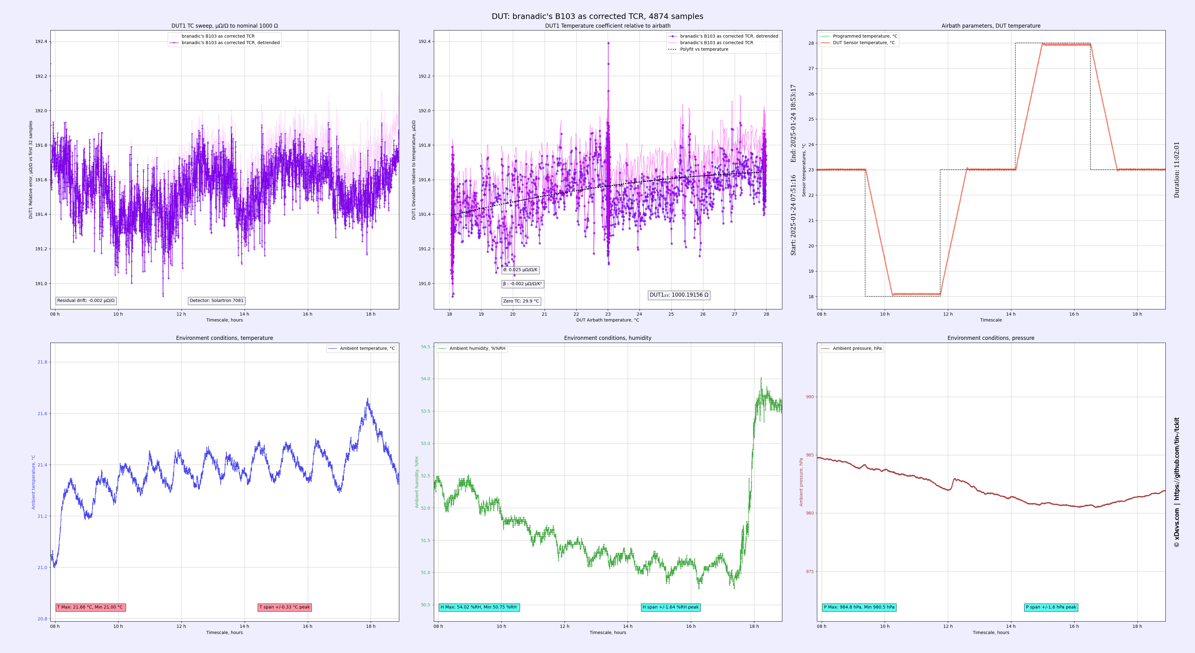
Figure 18: 1000 Ω analytics after first TCR trim

CSV-file with TCR data, VPG 1 kΩ element

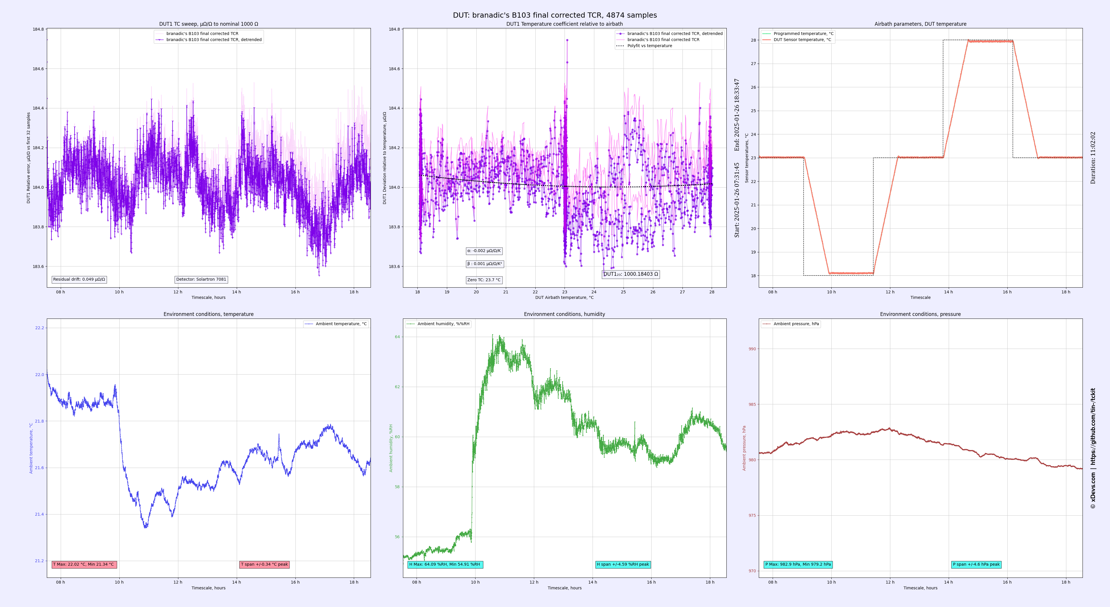
Figure 19: 1000 Ω analytics final TCR trim

xDevs.com analytics TCkit run with 10 kΩ element output

CSV-file with TCR data, VPG 10 kΩ element

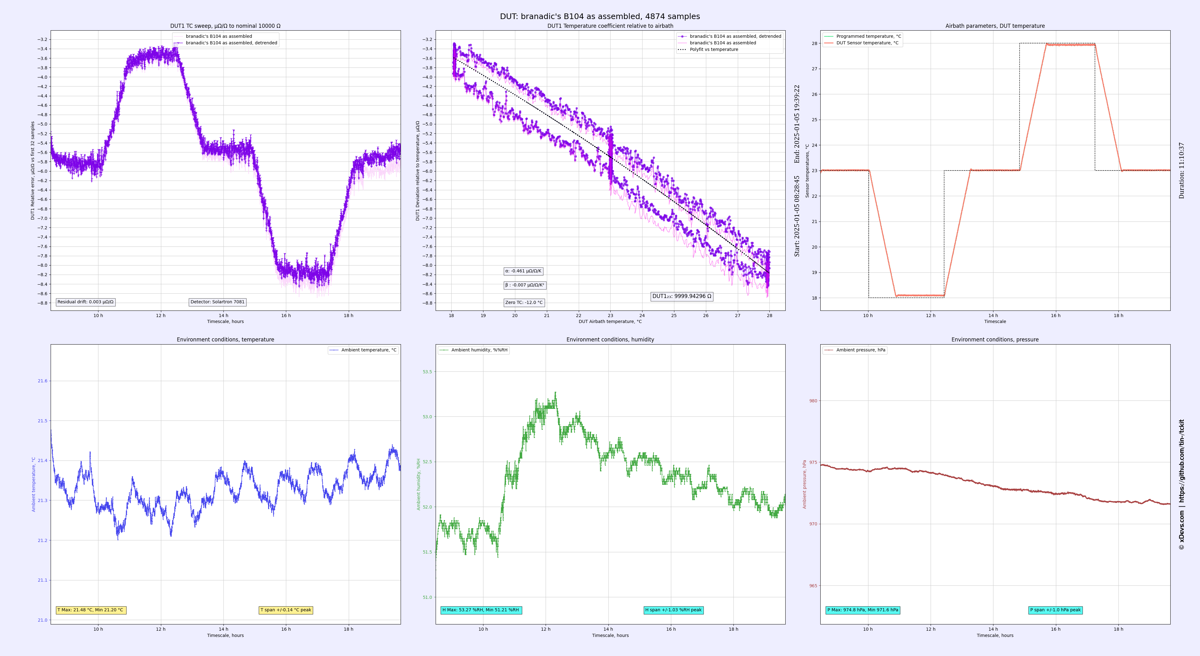
Figure 20: 10 kΩ analytics as assembled

CSV-file with TCR data, VPG 10 kΩ element

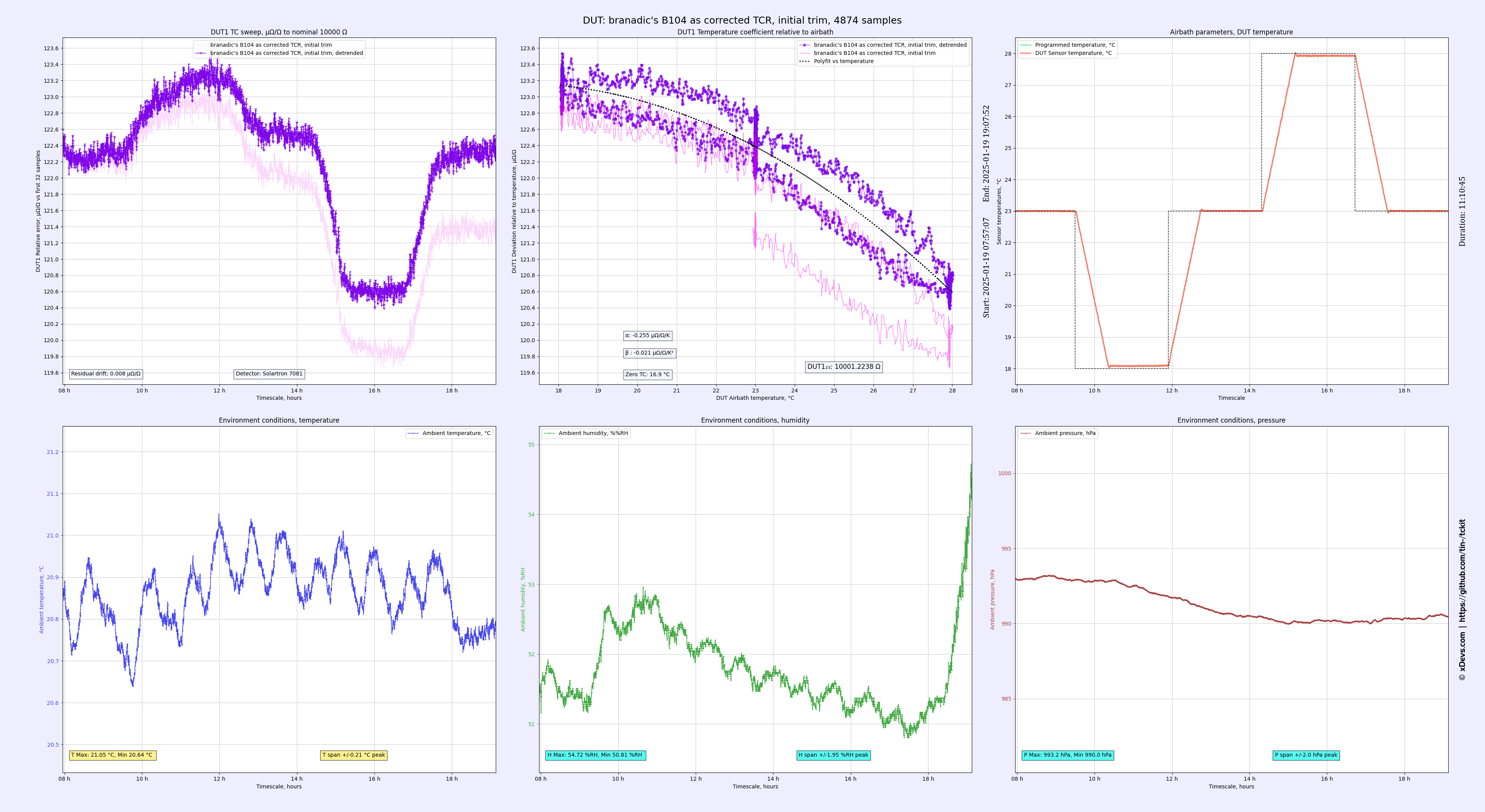
Figure 21: 10 kΩ analytics with correction, trim 1

CSV-file with TCR data, VPG 10 kΩ element

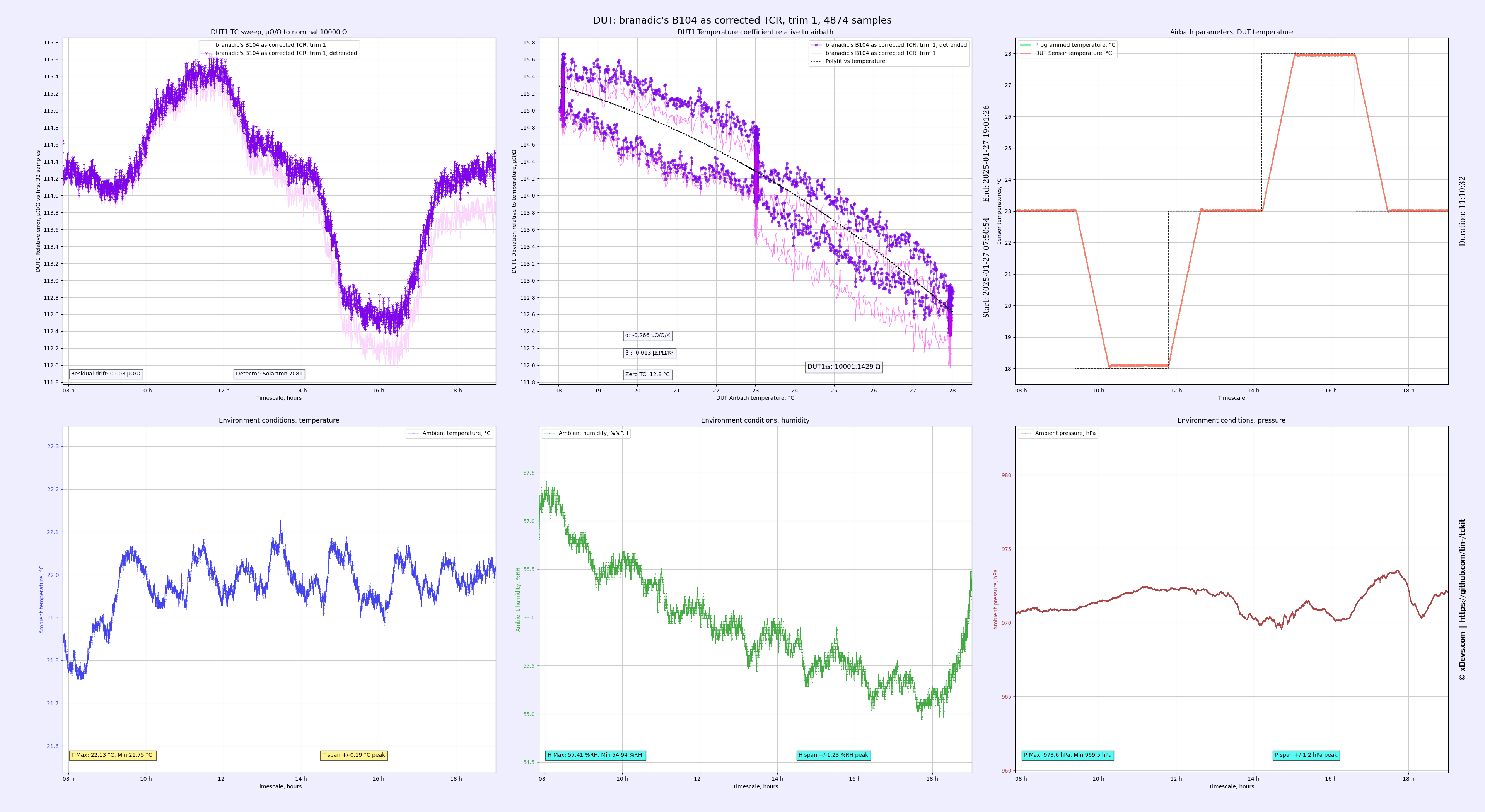
Figure 22: 10 kΩ analytics with correction, trim 2

CSV-file with TCR data, VPG 10 kΩ element

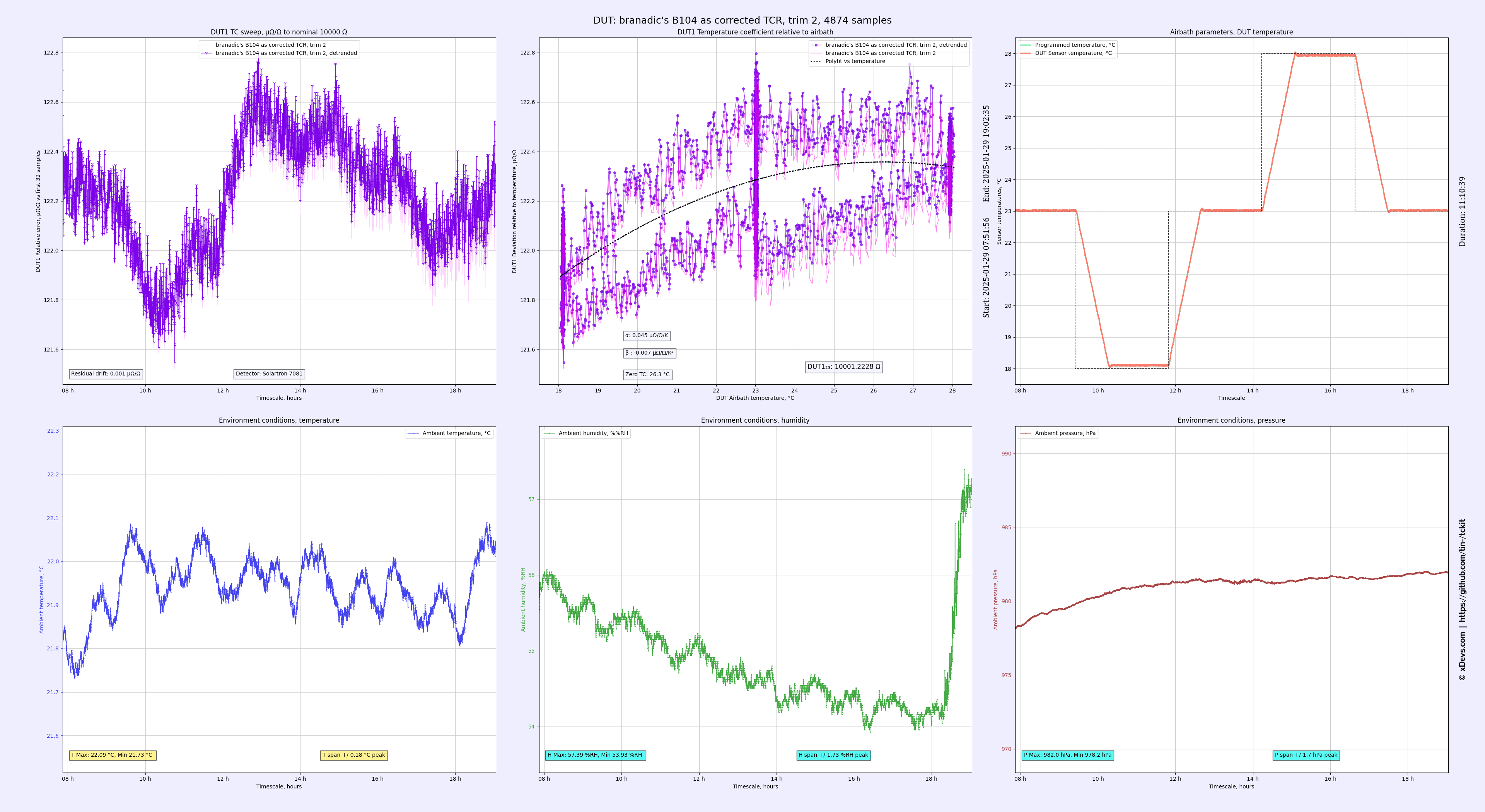
Figure 23: 10 kΩanalytics with correction, trim 3

CSV-file with TCR data, VPG 10 kΩ element

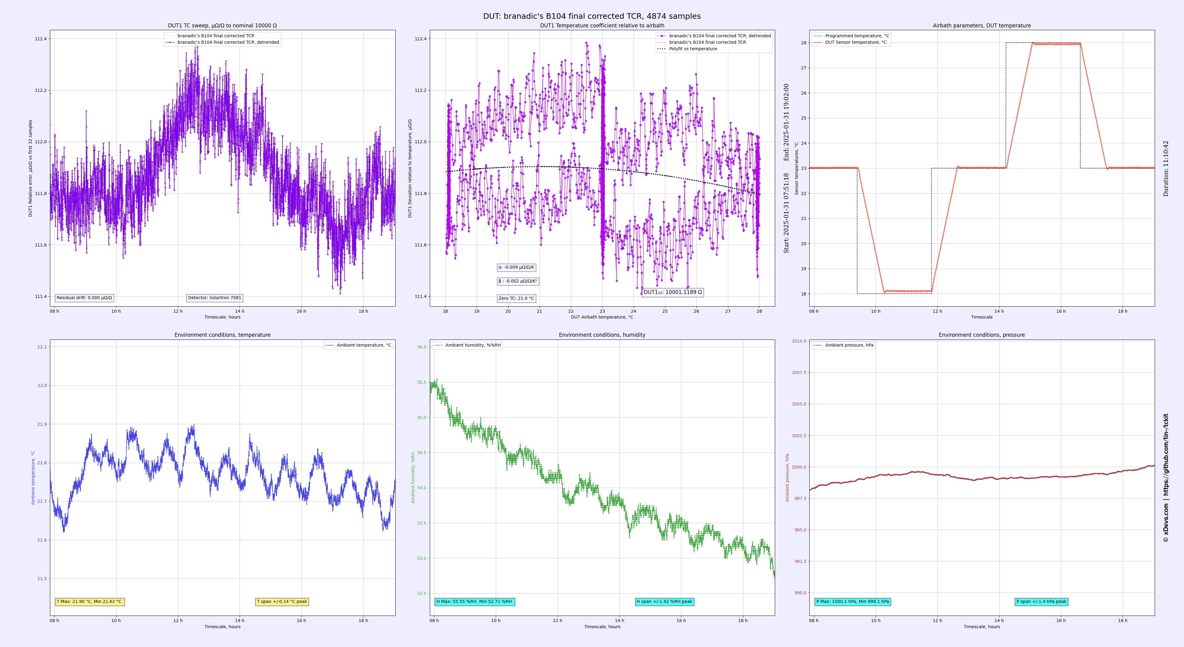
Figure 24: 10 kΩ analytics with correction, final trim

Resistor	Final TCR (original analysis)	Final TCR (xDevs TCkit numbers)	Difference for α and β
VHP202-100	αT23 = 0.013 µΩ/Ω/K , βT23 = -0.001 µΩ/Ω/K²	αT23 = +0.023 µΩ/Ω/K , βT23 = -0.002 µΩ/Ω/K²	10 nΩ/Ω/K, -1 nΩ/Ω/K²
VHP202-1k	αT23 = 0.0043 µΩ/Ω/K , βT23 = 0.0015 µΩ/Ω/K²	αT23 = -0.002 µΩ/Ω/K , βT23 = +0.001 µΩ/Ω/K²	-6.3 nΩ/Ω/K, -0.5 nΩ/Ω/K²
VHP202-10k	αT23 = -0.0103 µΩ/Ω/K , βT23 = -0.0048 µΩ/Ω/K²	αT23 = -0.009 µΩ/Ω/K , βT23 = -0.002 µΩ/Ω/K²	1.3 nΩ/Ω/K, 2.8 nΩ/Ω/K²

Table 5: Final α and β coefficients for the resistors obtained from TCkit

With these plots we can assign following calibration values for each of the outputs by this low-cost DIY resistance standard:

Resistor	Final value (original analysis)	Final value (xDevs TCkit numbers)	Relative difference
VHP202-100	100.03555 Ω	100.03557 Ω	-0.2 µΩ/Ω
VHP202-1k	1000.1841 Ω	1000.18403 Ω	+0.07 µΩ/Ω
VHP202-10k	10001.118 Ω	10001.1189 Ω	-0.09 µΩ/Ω

Conclusion

So there you have it, it is easy to compensate a resistors linear TCR just by using some additional copper wire in series to it. It’s no rocket science and easy enough to give it a try yourself.

If you are not happy with the result after the first try, keep trying again. Additional trimming of the copper wire and repetition of the temperature sweeps can be performed until the chaos comes home and the TCR curves are completely flat in the temperature range of interest. This is quite simple and powerful method and can be used for any resistance element that has negative temperature coefficient to begin with. With carefully selected compensation it’s possible to achieve TCR performance better than any 8½-digit DMM could measure over a typical laboratory temperature variations.

In case you need to compensate a second order term, also read the article [2] , which makes use of the non-linear behavior of a thermistor connected in parallel to the resistor to be compensated.

Discussion about this article and related stuff is welcome in comment section or at our own IRC chat server: irc.xdevs.com (port 4808, channel: #xDevs.com) or by reaching out by email.