- Introduction
- Disclaimer
- Metrology Glossary
- SI 2019 and its impact to electrical metrology
- xDevs.com’s current primary standards
- Cooperation with national level metrology lab, ITRI CMS NML, Taiwan
- Calibration results
- Transfer of voltage, using +10.000 V DC standard
- Transfer of resistance, using 10.000 kΩ resistance standard
- Artifact calibration verification of Keysight 3458A DMM tandem
- Summary and conclusion
Introduction
Every single piece of instrumentation we have today depends on accurate measurement of related quantity units. We need the accurate realization of second to time our processes and frequency in signals. Measuring devices, even simple voltmeter used to check car battery in the field or household power meter that counts how much to pay this month for electric power; speedometer that shows car speed – all calibrated to a more stable standard at some point during manufacturing. Those standards calibrated by higher-end references, and in the end traceable to international SI unit.
To ensure agreement between measurement results of all possible physical parameters, people in 1875 started development and use of the single metric system, known today as The International System of Units. This SI metric system applied worldwide to ensure that products developed across the world are measured the same way and have the same quality. If you buy 1 kilogram of gold from France bank to sell in Australia, SI ensures than a bank in Australia also accounts it as 1 kg of gold, not 980 gram or 1010 gram. Every person who ended up with metric screws but imperial nuts already know why a single system is very important :).
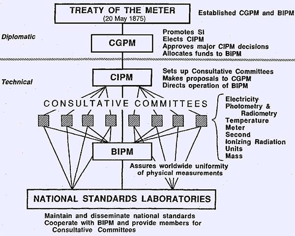
Image 1: International Metrology Organization Hierarchy
SI defines 7 base units, ampere, candela, kelvin, kilogram, meter, mole and second. Other derived units are defined in relation to these seven base units. The base units are derived from intrinsic constants of nature, like the speed of light in vacuum or charge of the electron, which is observed and measured with great accuracy by international research teams and scientists. With carefully defined units, measurements of practical standards and artifacts existing today are possible to uncertainty better than a few parts per billion. In percentage units that is tiny 0.0000001%! So the reader may ask, why such measurement accuracy is so important, and why engineers may need to know a quantity with 0.0000001% accuracy? Well, this question is not simple.
People of the modern industrial world are surrounded by tools and machines, to aid labor and improve living. This advancement and progress depend on the quantified measure of physical units and parameters, that allow us to compare and correctly test our ideas, tools, machines, and products. Take the unit of time as an example. Let’s assume you are traveling and have a plane ticket, with departure time 14:00 precisely. Airport schedule maintained by high accuracy clocks and for simplicity, we assume all of the airport services done and plane ready exactly on time. However, because of the mechanical shock calibration of your watch starts running faster and reported time to become off by 30 minutes, but you did not notice it. You arrive at the airport gate for departure, 13:40 according to the watch, only to find out that the airplane just left 10 minutes ago. This is an exaggerated example of what happens if “your” second and “airport” second are not in close agreement. Today this example sounds impossible with the number of smartwatches, airport clocks and requirements to arrive at the gate well in advance, but in not so distant past such example could be well possible in real life.
Another time example is cellular phone and wireless network application. These systems rely on the very accurate time realization, so your pocket smartphone expects signal at frequency Y and cell base station tower antenna need to transmit signal very close to that frequency Y, otherwise the phone will not “hear” the station and cease to get reception. Hence most of the wireless cell stations are using very stable atomic Rubidium-disciplined clocks, maintaining the correct time and frequency, often with an error less than 2 × 10-12 to maintain frequency alignment.
The correct measure of a second is important to know the exact speed of the vehicle like an airplane or car. If the speedometer showing incorrect value with large unchecked error, that could lead to an accident and even cost human lives.
Perhaps car speed is not requiring measurement with 0.0000001% accuracy. Speedometer in the car may have accuracy just 1%. However, speedometer manufacturer must verify and certify that each meter leaving production line indeed meets 1% level accuracy. This is possible when the production line has own speed measurement accuracy better, for example at 0.1%, to provide an accurate test for each speedometer device under test (DUT). But how the factory can know they use 0.1% accurate equipment? To resolve this question, the factory will send their equipment to industry calibration lab, shown by metrology hierarchy triangle on Image 2. This next level calibration lab that test production line equipment must have accurate methods to test speed with an error of less than 0.01%. Still, the task is not over here and measurements eventually build a long chain of labs and results, till the direct comparison with the realization of base or derived SI units at national and international level for the final traceable calibration step.
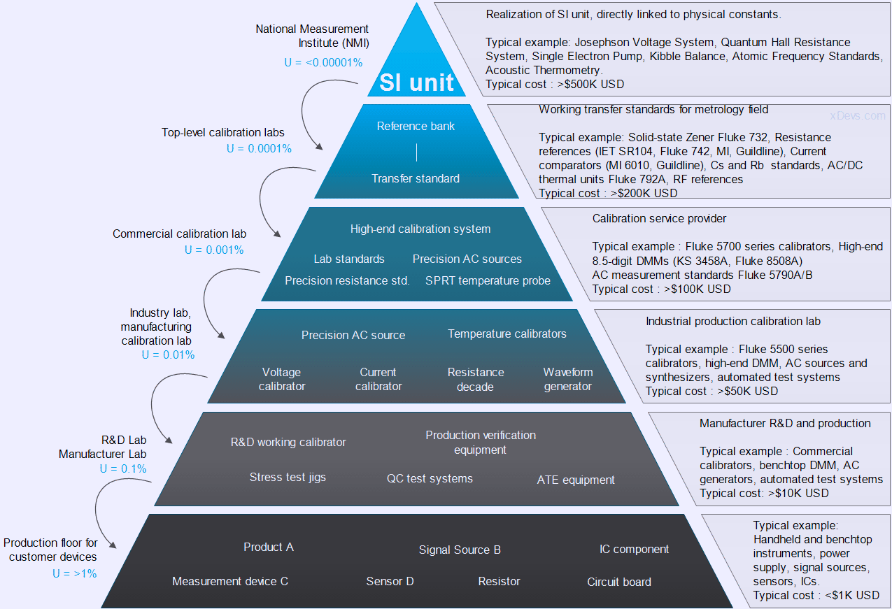
Image 2: Example calibration hierarchy and conceptual relation between levels for voltage and resistance
In other words – every measurement always has error. Traceability and calibrations provide a way to estimate the magnitude of that error. Measurements performed on a higher level, closer to SI unit implementation, performed with higher grade equipment can offer better measurement uncertainty (smaller error of measurement) and account for more error factors.
However, cost of making better measurements increase a lot as well, requiring more time and more expensive delicate equipment with severe maintenance and operation costs, especially compared to typical commercial level calibrators and sources. With every next level amount of factors that must be accounted for measurement uncertainty budget are multiplying, transforming total error estimation into difficult statistics and the time-correlated math task. Add labor costs, logistics, no wonder why cost goes in magnitude when you jump into next decimal digit of accuracy in measurement. There are thousands of meters that provide 1% or even 0.1% accuracy levels, but only a handful of expensive instruments and manufacturers that can offer 0.001% accuracy.
Table 1 and 2 illustrate the same concept but in different presentation format, highlighting difficulty and resource required for desired accuracy and stability level.
| SI unit | Desired resolution | Desired accuracy | Implementation cost | Device example |
|---|---|---|---|---|
| DC Voltage | <3½ digits | 1% | <$10 USD | Handheld or industrial DMM / Voltmeter, integrated MCU ADC |
| DC Voltage | 4½ digits | 0.1% | ~$100 USD | High-end handheld DMM, entry level benchtop DMM |
| DC Voltage | 5½ digits | 0.01% | $500 USD | Bench-top DMM, high-performance 24-bit ADC, calibrators |
| DC Voltage | 6½ digits | 0.001% (10 ppm) | $5,000 USD | High-end benchtop DMMs, high-end calibrators, 32-bit ADC |
| DC Voltage | 7½ digits | 0.0001% (1 ppm) | $20,000 USD | Best metrology DMM (Keysight 3458A, Fluke 85×8, Datron 1281) |
| DC Voltage | 8½ digits | 0.00001% (0.1 ppm) | $50,000 USD | DC reference bank with nanovolt-meter detectors and KVD |
| DC Voltage | Primary Quantum standards, >9½ digits | <0.05 ppm | $500,000+ USD | JVS , liquid helium cooled or dual-stage cryocooled |
Table 1: Voltage system levels and implementation for desired levels of accuracy
Take a note and think for a second, why expensive commercial 8½-digit DMMs like 3458A, 8508A/8588A or K2002 are considered only 7½-digit here. This is not a typo, and number have very obvious reason for it.
Another important note, resolution is not equal to accuracy, these two terms and parameters are in fact have very different meaning. Resolution defines what is the smallest change of the signal can be detected and quantified by the measurement, while accuracy define the total error of the measurement, compared to the unit definition.
| SI unit | Desired resolution | Desired accuracy | Implementation cost | Device example |
|---|---|---|---|---|
| Resistance | <3.5 digits | 1% | <$10 USD | Typical precision resistors, hand-held DMM |
| Resistance | 4.5 digits | 0.1% | ~$100 USD | High-end handheld DMM, entry level benchtop DMM |
| Resistance | 5.5 digits | 0.01% | $700 USD | Bench-top DMM, high-end precision resistors, resistance decades |
| Resistance | 6.5 digits | 0.001% (10 ppm) | $5,000 USD | Top-end benchtop DMM, resistance calibrators, resistance references |
| Resistance | 7.5 digits | 0.0001% (1 ppm) | $30,000 USD | Resistance bridges and ratiometric setups with Fluke 85×8, Datron 1281 |
| Resistance | 8.5 digits | 0.00001% (0.1 ppm) | $100,000 USD | High-end bridge and reference primary standards |
| Resistance | 9.5+ digits | 0.000005% (0.05 ppm) | $300,000 USD | DCCT top end bridges |
| Resistance | Primary intrinsic standard, >10+ digits | <0.02 ppm | $600,000+ USD | QHR System, CCC, liquid helium or dry cryocooler |
Table 2: Resistance system implementation, and levels of accuracy
Now the top base SI units are updated and at International Metrology Day – May 20, 2019 new SI units become effective, moving away from human-made artifacts. Aging/drift errors in artifact standards can no longer impact SI unit definition after May 20, 2019.


Image 2-3 : SI system units before (left) and after 20 May 2019 (right). Credits .
Gray circles on old SI graph represent physical artifacts, such as International Prototype of the Kilogram MIPK or triple point of water, +0.01 °C T[~TPW]. These artifacts produce extremely stable reference values, but being non-ideal macroscopic objects, they are not constant and still drift by tiny, yet detectable amount.
Change of the SI unit, in theory, affects complete hierarchy and all previous calibration results, but in practical applications deviation is so small, that even top-level calibration laboratory might not be able to see the difference between previous SI and new SI. There is no need to worry about measurement error in typical handheld DMMs or power supplies because their own stability and accuracy are magnitudes worse than the induced deviation from new SI 2019. We expect that redefinition in SI units would only affect measurements by national measurement laboratories and international scientific research projects that work with top-notch instrumentation to detect sub-ppm (<0.0001%) change, and not affect most commercial applications.
To celebrate this major change xDevs.com project team finally committed to obtaining direct voltage and resistance calibration transfer to National Level Quantum standards. This is not as easy as may sound, so this article only covers these two derived units, volt V and resistance Ohm (Ω). SI units’ redefinition makes 2019 special year, as the last change of similar significance for voltage and resistance was 29 years ago with the implementation of SI-1990 change for Volt and Ohm. Cooperation with Taiwan’s key National Measurement Laboratory (NML), Industrial Technology Research Institute made this calibration service and this article possible.
Voltage and Resistance are derived units from redefined Ampere . The ampere, symbol A, is the SI unit of electric current. It is defined by taking the fixed numerical value of the elementary charge e exactly 1.602176634 × 10⁻¹⁹ when expressed in the unit C, which is equal to A s, where the second is defined in terms of ΔνCs.
Disclaimer
Redistribution and use of this article, any parts of it or any images or files referenced in it, in source and binary forms, with or without modification, are permitted provided that the following conditions are met:
- Redistributions of the article must retain the above copyright notice, this list of conditions, link to this page (https://xdevs.com/article/si2019/) and the following disclaimer.
- Redistributions of files in binary form must reproduce the above copyright notice, this list of conditions, link to this page (https://xdevs.com/article/si2019/), and the following disclaimer in the documentation and/or other materials provided with the distribution, for example, Readme file.
All information posted here is hosted just for education purposes and provided AS IS. In no event shall the author, xDevs.com site, ITRI CMS or any other 3rd party be liable for any special, direct, indirect, or consequential damages or any damages whatsoever resulting from loss of use, data or profits, whether in an action of contract, negligence or other tortuous action, arising out of or in connection with the use or performance of information published here.
If you willing to contribute or add your experience regarding the testing performance of various instruments or provide extra information, you can do so following these simple instructions.
Metrology Glossary
There are multiple documents and guides available online that explain defined methods and processes in metrology, which are key for calibration principles, such as:
GUM: Guide to the Expression of Uncertainty in Measurement
International Vocabulary of Metrology – Basic and General Concepts and Associated Terms
- Calibration – operation that, under specified conditions, in a first step, establishes a relation between the quantity values with measurement uncertainties provided by measurement standards and corresponding indications with associated measurement uncertainties and, in a second step, uses this information to establish a relation for obtaining a measurement result from an indication. Calibration does NOT mean adjustment or altering of the standards output.
- Calibration interval – time between calibrations of the standard. Can be any value, but often used values are 1 year, 180 day, 90 day or 24 hour period. Often specifications provide uncertainty for multiple calibration intervals.
- Measurement uncertainty – non-negative parameter characterizing the dispersion of the quantity values being attributed to a measurand, based on the information about measurement.
- Uncertainty budget – statement of measurement uncertainty, of the components of that measurement uncertainty, and of their calculation and combination into total measurement error.
- Standard measurement uncertainty – measurement uncertainty expressed as a standard deviation
- Metrological traceability – property of a measurement result whereby the result can be related to a reference through a documented unbroken chain of calibrations, each contributing to the measurement uncertainty
- National measurement standard – measurement standard recognized by national authority to serve in a state or economy as the basis for assigning quantity values to other measurement standards
- Coverage factor – number k > 1, by which a combined standard measurement uncertainty is multiplied to obtain an expanded measurement uncertainty.
- Transfer standards – device that generates stable output, which they can be calibrated traceable to SI unit realization. High stability and robust construction are very important, to provide measurements valid over calibration interval.
- Drift – change in the device output or measurement, derived from internal or external factors. Factors include temperature, humidity, pressure variations, loading changes, mechanical tear&wear, internal parasitics in assemblies, PCBs, semiconductors, insulation leakage, stray electromagnetic fields, and many more.
SI 2019 and how electrical voltage and resistance are defined
Voltage is the potential difference between two points in the electric circuit. The amount of difference, expressed in units Volt (symbol V) indicate amount of potential energy that moves electrons from one point in the circuit to another. As result voltage identifies how much work, potentially, can be done through the electric circuit. If we imagine an electric conductor as the water pipe, the voltage would be the diameter of the pipe. Voltage unit is named after physicist Alessandro Volta (1745-1827), who invented the voltaic pile – ancient equivalent of the today battery cell.
Resistance is a measure opposite to current flow in an electrical circuit. It is expressed in units Ohm (symbol Ω). With same voltage in the circuit, a higher resistance in the path will reduce the amount of electron flow (current), while lower resistance would increase current flow. If we imagine an electric conductor as the same water pipe, resistance equivalent would be amount of valve opening. Ohms are named after physicist Georg Simon Ohm (1784-1854) who studied the relationship between voltage, current and resistance and formulated famous Ohm’s Law.
If we extend the water pipe example to Current, that is the amount of water, flowing thru the pipe. Current is expressed in units Ampere (symbol A). Current defines the number of electrons flowing past a point in a circuit over a given time. A current of 1 Ampere means that 1 coulomb (6.241509126(38) × 1018 electrons) is moving past a single point in a circuit per 1 second.
Voltage SI Volt unit
Here we will touch on SI unit redefinition 2019 in terms of voltage and resistance and practical impact on the calibration applications. SI unit volt (V) realized using the quantum Josephson effect discovered in 1973, with the help of the cryogenic system and the new value of the Josephson constant.
KJ = 2e/h = 483597.848416984 GHz V-1
From SI redefinition elementary charge e is now equal 1.6021766341 × 10⁻¹⁹ coulomb exactly, and Planck constant h is 6.626070150 × 10⁻³⁴ J Hz-1 exactly. The advantage of new value of KJ for practical use is that it ensures that virtually all realizations of the volt unit, based on the Josephson effect will provide exactly the same result.
Old pre-2019 value, which was adopted by CIPM starting 1 January 1990 KJ-90 = 483597.9 GHz V-1 is larger by the fractional amount 106.665 ppb(parts per billion). This implies that the new unit of voltage realized after 20 May 2019 using updated KJ now smaller by the same fractional amount -106.665 ppb.
This small, but detectable change would affect only highest-precision calibration systems, used in top-level labs that obtain and maintain calibrations with fractional 10-6 (1 ppm) uncertainty for DC voltage. Other than JVS system itself, a typical example of such realizations are predicted reference voltages from banks of four or more Fluke 732 (734A/C), Datron 4910 series and Wavetek/Fluke 7004/7010N series arrays, that are constantly powered and monitored for on-site lab’s Volt value. In more practical cases, even very expensive 8½-digit DMMs like Keysight 3458A or Fluke 8508A such small change would be already masked by their own zener reference noise, thermal coefficient, and errors of the measurement path and ADC.
Resistance SI Ohm unit
The unit of resistance, ohm Ω can be realized by using the Quantum Hall effect and the following new value of the von Klitzing constant RK.
RK = h/e2 = 25812.8074593045 Ω
Old value RK-90 = 25812.807 Ω was adopted by the CIPM starting 1 January 1990 for the international realization of the Ohm. Change of the new RK is the fractional amount +17.793 ppb(parts per billion). This implies that the unit of resistance realized after 20 May 2019 using new RK is larger by the same fractional amount. Previously on January 1, 1990 USA unit of resistance was adjusted by +1.69 ppm when US Legal Ohm was redefined in terms of QHE realization.
This change can be detected only by direct current comparator bridges and ratiometric systems, so for practical commercial calibration labs change of SI resistance unit have a smaller impact than voltage, because the annual drift of best conventional resistance standards is usually worse than this deviation. Impact from Ohm unit change is even less than voltage, so this has a minimal practical impact on commercial calibration labs and their operations.
These formulae and calculations look simple and easy, but in real life many NMIs and collaborations worked years, if not decades to establish a direct connection between the fundamental physical constants and macroscopic experiments to provide transfers and comparisons to have traceable uncertainty less than 10-8 or better. These efforts allowed the international metrology community to move from human-made artifacts definitions in 2018-2019 to basic constants of nature. universal for the world. Eventually old international artifact standards like International Prototype of the Kilogram will find their place in museum as important history piece.
BIPM also has released guidance document regarding impact from redefined SI units for voltage and resistance.
xDevs.com labs primary standards, used as reference sources
How that theory is briefly covered, we can move to the practical experiments and calibrations. xDevs.com have two equally important private labs, located in the USA and Taiwan, where most of the test equipment you see on this site is tested and fixed. Lot of gear setups between both labs similar and overlapping in voltage and resistance capability. Both labs running daily for educational and research purpose, to study metrology-relevant topics, such as stability of the solid-state zener reference designs, resistance standards testing, various experiments to explore instrumentation limits and perform data analytics for precision applications.
As part of the lab maintenance, we do internal instruments repair and calibration in-house, including extensive component level and custom electronics hardware development. Most of the equipment controlled 24/7 with in-house Python software, running on dedicated data collection computers such as Raspberry Pi and GPIB networks. Covering complete lab details is outside of this article scope, however, it is important to note key primary DC and resistance standards used as calibration references for all underlying transfers.
TW Lab primary standards set
Fluke 732B – 10 VDC and 1.018 VDC output reference. Industry-proven DC voltage standard, widely used by many calibration and metrology labs all around the world. Usually able to deliver stability better than ±2 ppm a year with predictable linear drift.
In theory any source, even generic battery cell can be calibrated (measured) with use of the highest precision system, however that exercise does not have many purposes as tested device drifts outside of measurement uncertainty very fast. Multiple stable calibration sources are often used at metrology labs for redundancy and cross-verification. If an ensemble of four references is holding accurate value, according to statistics, it is less likely that all four would drift same way. If any single reference in bank start showing unexpected behavior due to electrical or physical damage/stress this can be detected by comparing to other references, even before the next calibration cycle to SI Volt transfer.
Also ambient and standard temperature, humidity, pressure, loading current and even type of cable and physical stress on chassis are affecting output value of the standard. To reduce the impact of temperature and humidity most of commercial DC Voltage references equipped with built-in temperature ovens that maintain solid-state special circuit and critical components. These ovenized references such as Fluke 732 series have backup battery power, which limits shipping/transit time and impose regulations on safety.
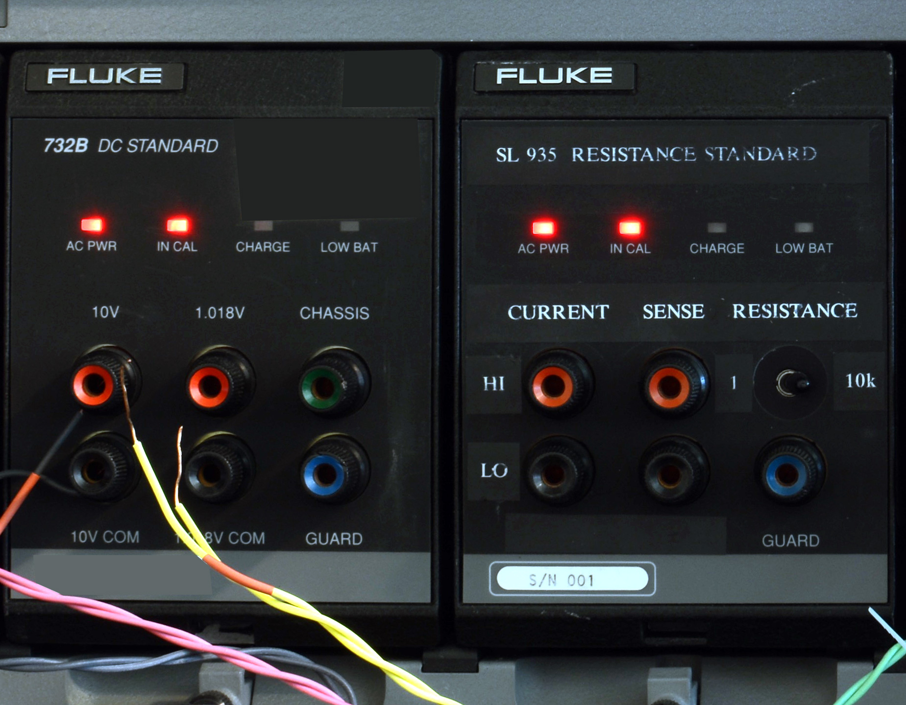
Image 4: Fluke 732B and prototype Fluke SL935 standards
Prototype Fluke SL935 ovenized resistance standard , with 1 Ω and 10 KΩ output. This prototype device build by secret Fluke lab, using hermetic thin-film laser trimmed resistor networks from no less than ten (!) Fluke 5720A calibrators to obtain ultra-low temperature coefficient and stability for both output values. Unit is built around 732B reference chassis, replacing original DC Voltage reference electronics with custom resistance module. Oven operating at reduced temperature, fixed around 40 °C to reduce annual drift.
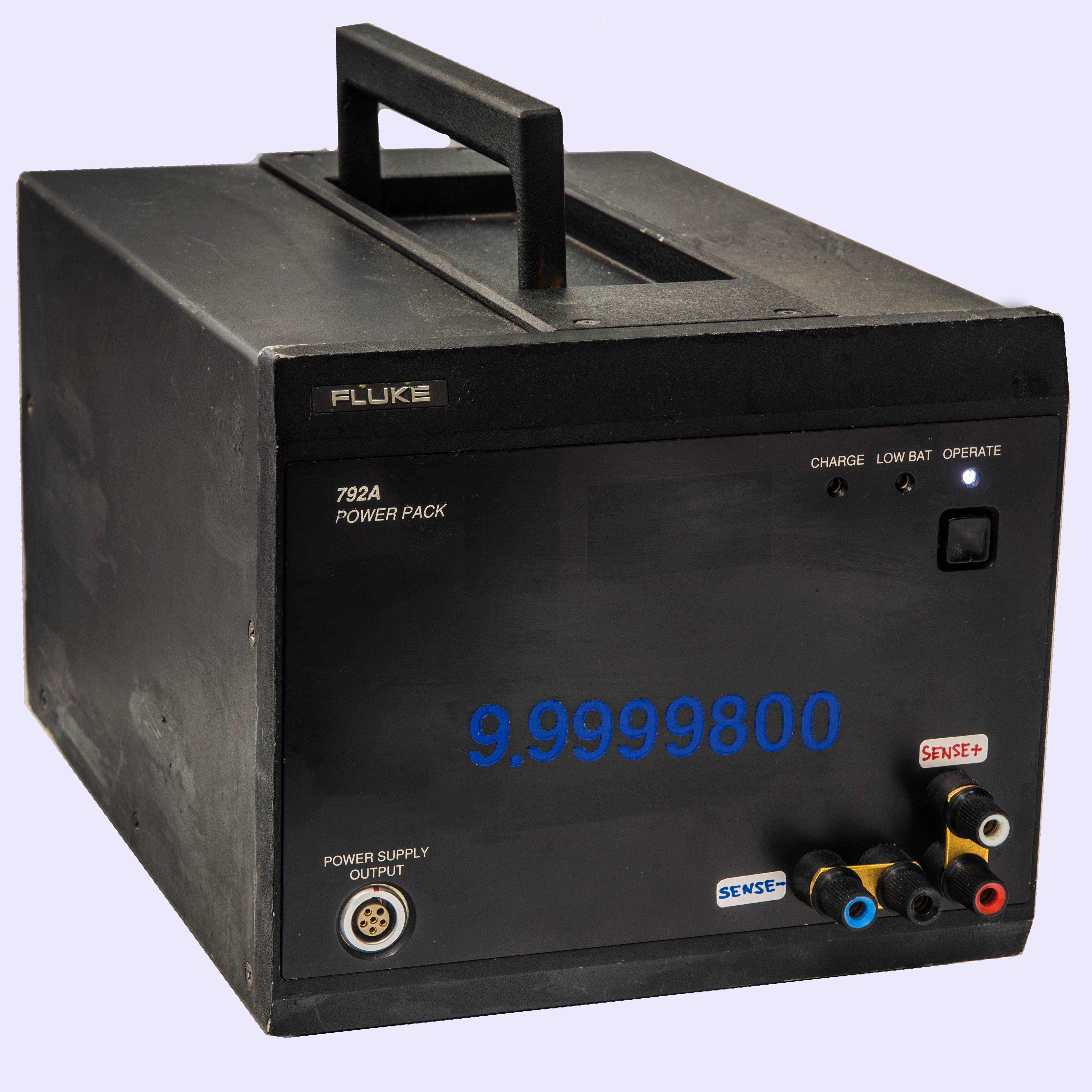
Image 5: DC Voltage reference 792X based off modified Fluke 792A Power Pack
Over last few years here at xDevs.com lot of experiments were completed with our own custom designs in search of the ultimate stability DC voltage reference. Most of these utilize best reference on the market – Analog Device (former Linear Technology) LTZ1000 and LTZ1000A Super-Zener. Some publications about these designs available here, here and here. These designs demonstrated short-term stability well within under 1 ppm over period of days/weeks, with errors mostly induced by environment and measurement setups, rather than reference itself.
One such prototype xDevs.com 792X FX LTZ1000A reference, assembled in Fluke 792A Power Pack. This standard provides +10 VDC nominal, with estimated annual drift less than -3 ppm. Key feature is high output drive capability with minimal loading errors, due to use of true 4-wire Kelvin connection output. Unlike Fluke 732B, this unit is able to sink or source currents up to 25 mADC with minimal error to the output voltage.
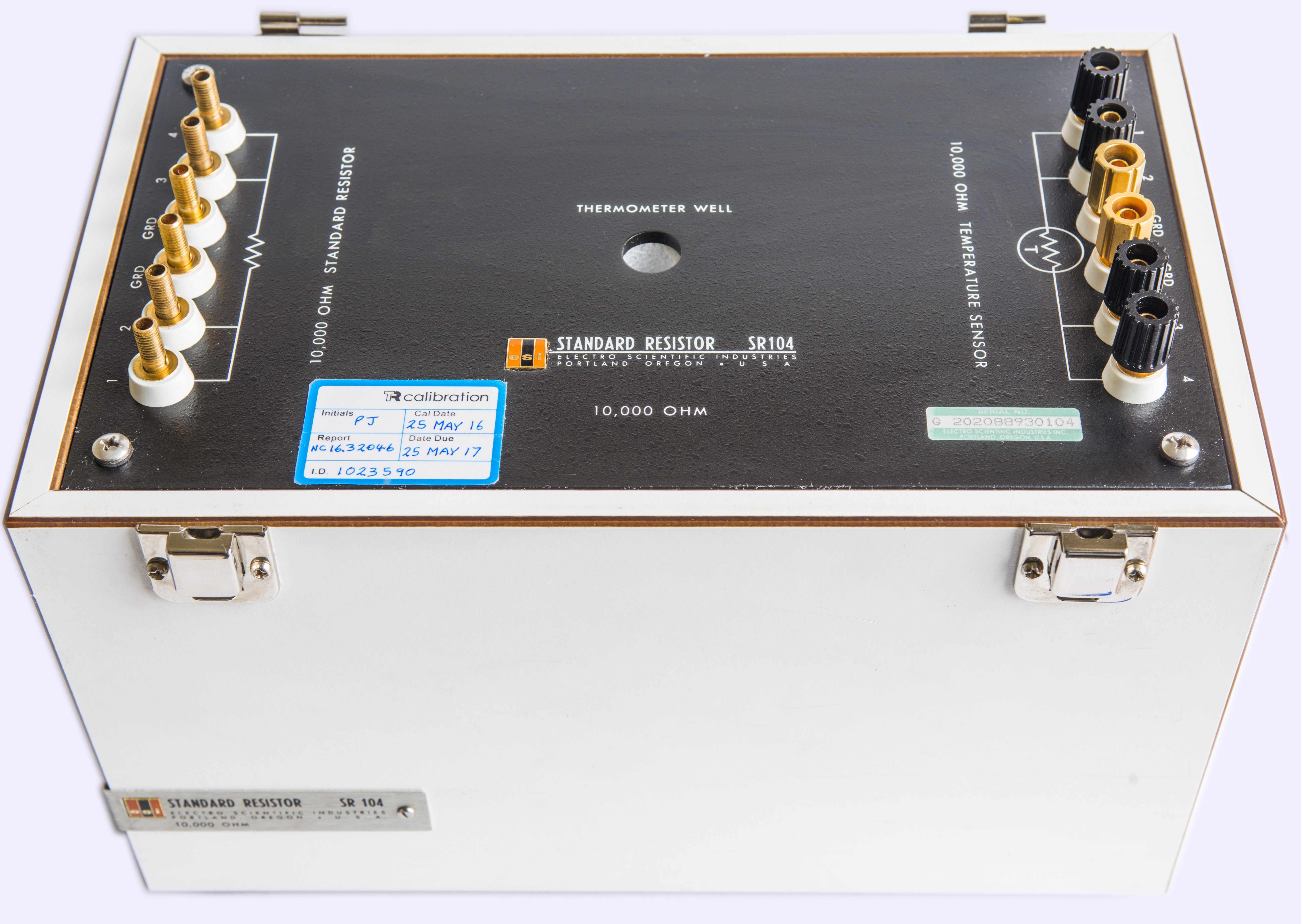
Image 6: ESI SR104 hermetic 10000 Ω primary resistance standard
ESI SR104 – resistance standard with the ultra-stable resistive element, temperature sensor, all enclosed in a sealed oil-filled metal can. Everything is embedded in nice wooden box (there is an option from IET without wooden enclosure as well). ESI, being one of the industry original experts in resistance field, invented and designed legendary SR104 10000 Ω resistance standard in 1967, considered as metrology primary level grade product by many labs. This standard is still unrivaled on the market, 52 years since. Perhaps that shows how hard it is to make improvements on high-end metrology instrumentation. For fun comparison – Intel 4004 processor, released well 4 years after ESI SR104 evolved into modern 56-core+ monsters on 14nm process.
Often units with original manufacturing date codes before 1990 are still found within specifications. Thanks to rugged construction and own oil tank, these standards are not subjected to humidity variations and can provide ~0.2 ppm resistance accuracy after careful tempco compensation using an integrated sensor resistance element. TEGAM has acquired resistance products from ESI, which in turn by the year 2006 were sold to IET Labs Inc.
IET Labs now still offer these resistance standards together with A2LA accredited calibration services covering not just SR104 but all complementary resistance, inductance, and capacitance standards. Along with SR104 Primary Standards Resistors other models are also maintained, such as 100 Ω SR102, SR1010, SR1030, SR1050 Working Resistance Standards, SR1 Decade Boxes RS925D, DB62, DB877 Kelvin Varley Dividers DP1211-DP1311, 242D, 240C bridges.
Modern day IET SR104 however is not the same standard as designed by ESI, and original special wire wound element was replaced by number of modern bulk metal foil elements, so new IET SR104 long term stability (years) will remain to be proven.
Datron (later Wavetek) Model 4920 is AC Voltage measurement standard, which is essentially a high precision voltmeter, but designed with the sole goal to perform accurate AC voltage measurements. After Datron/Wavetek instrumentation division acquisition by Fluke in early 2000’s this AVMS was discontinued and replaced by Fluke’s 5790A AC Measurement Standard. Still, some of the specifications and ranges are better than 5790A.
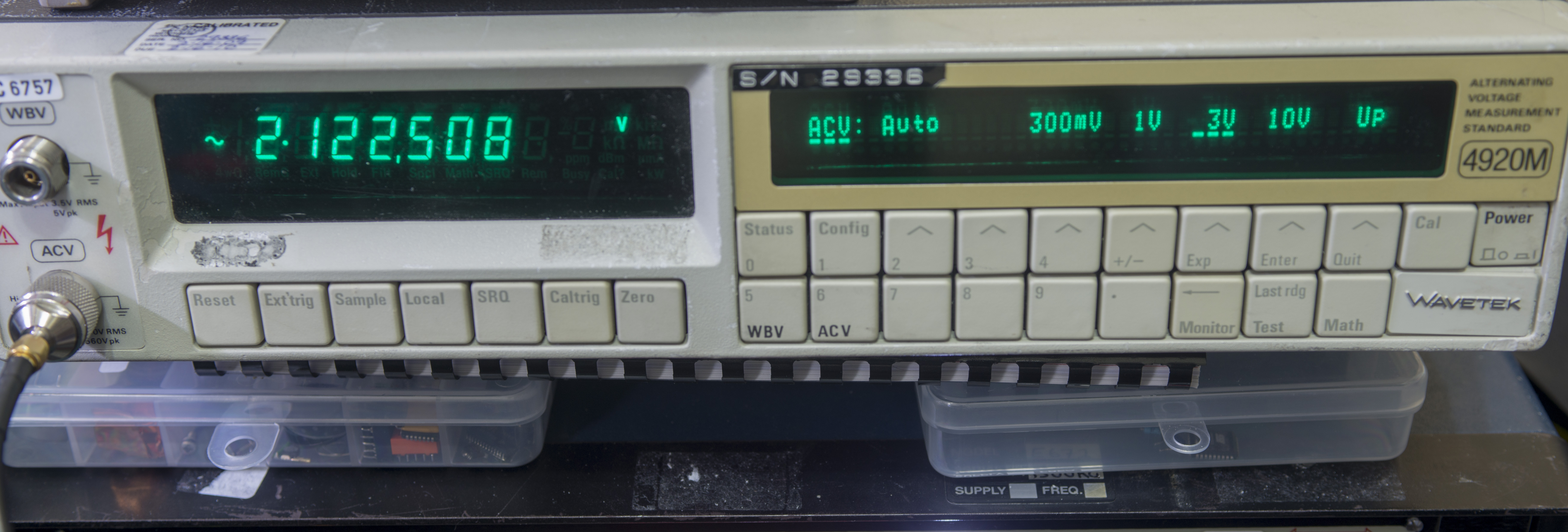
Image 7: Wavetek 4920M AC Voltage Measurement Standard
Two modified HP 3458A, calibrated to in-house 10V DC reference and 10 KΩ reference as linearity/transfer standard. The modification involves reduced oven temperature for primary reference to improve long-term stability. First unit (GPIB address 3) was repaired and in service since January 2016. The second unit (GPIB address 2) was repaired and adjusted by USA lab, put in service since February 2017. Both instruments are running powered up constantly 24/7 and used as verification references and linearity standards.
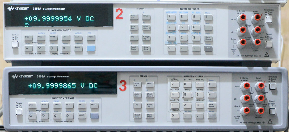
Image 8: Two modified Keysight 3458A 8½-digit DMMs
Fluke 5720A/03 calibrator with Fluke 5725A amplifier as working standard.
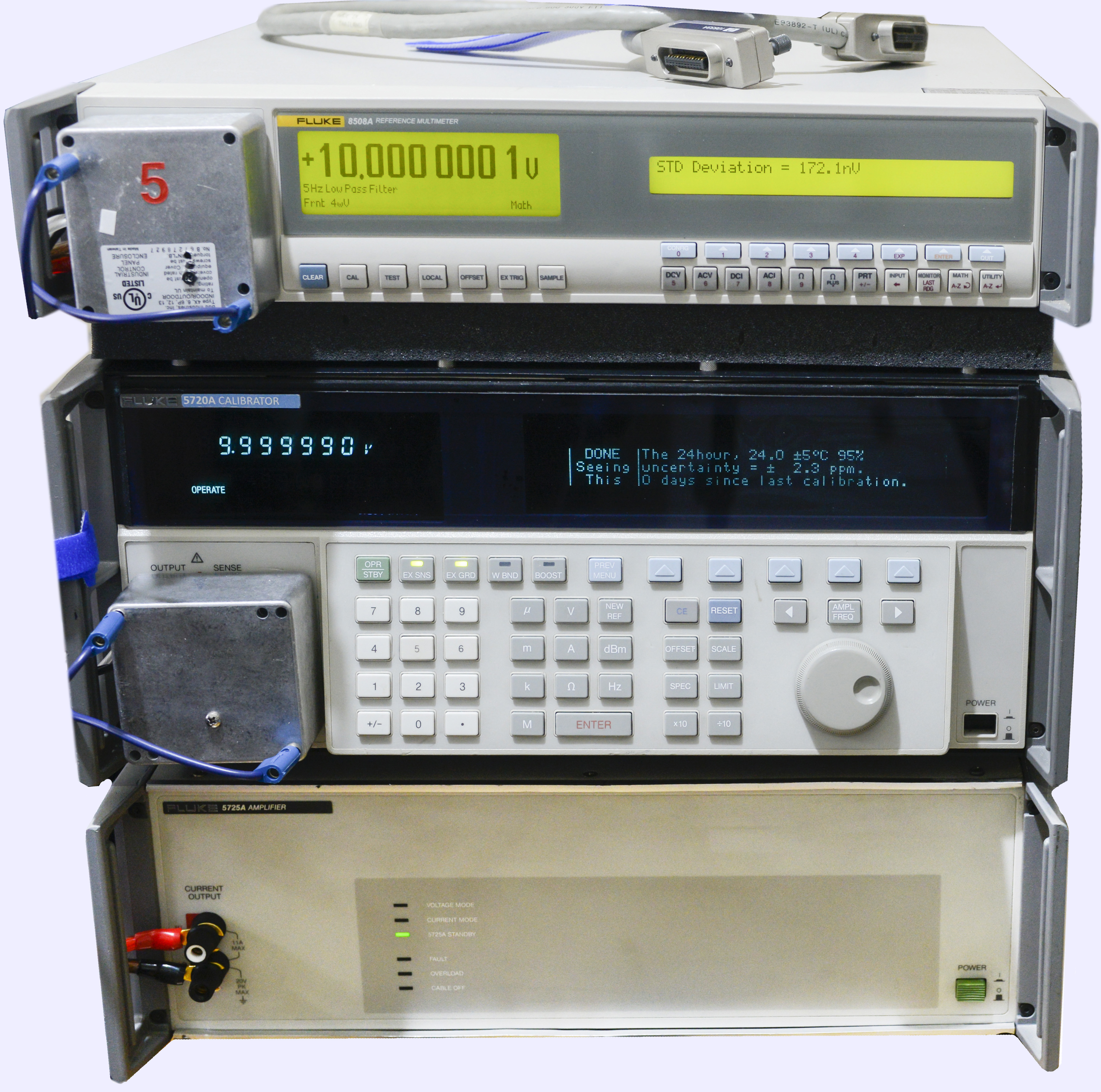
Image 9: High-performance calibration station with Fluke 5720A and Fluke 5725A
To transfer cardinal voltage, resistance and current points into arbitrary values with high stability and excellent linearity we use restored and fully optioned up multi-function high-end calibrator. Few additional calibrators, such as 5700EP and Datron 4808 are also used as auxiliary units for complex experiment setups, where more than one high-stability source could be needed.
Two TEMEX Rubidium atomic clocks and Trimble GPSDO module. These are in charge as frequency standards to provide precise 10 MHz to signal generators/analyzers and phase-lock for Fluke 5720A calibrator in ACV/ACI tests.
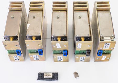
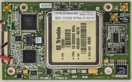
Image 10-11: Frequency GPSDO reference and atomic clocks with Rubidium cells
For calibration work this lab also have Fluke 752A Reference divider, multiple Fluke 720A KVD, Keithley 155 null-meter, Keithley 2182A and 1801/EM A10 nanovoltmeters, Fluke 5450A resistance calibrator, Keysight B2987A Electrometer/High-resistance meter and so on.
| Function | Instrument / standard | Key specification by manufacturer | Self-calibrated instrument |
|---|---|---|---|
| Source DC Voltage, 10 V | Fluke 732B , xDevs/Fluke 792X | ±3 ppm/year, <0.05 ppm/K TC | No |
| Source DC Voltage 1 mV – 1000 V | Fluke 5720A, Fluke 752A | ±2.5 ppm/year, relative to lab Volt | Yes |
| Source Resistance, 1 Ω | Fluke SL935 | ±3 ppm/year, <0.01 ppm/K TC | No |
| Source Resistance, 10 kΩ | ESI SR104, Fluke SL935 | ±0.5 ppm/year, <0.1 ppm/K TC | No |
| Source Resistance, 1 Ω – 100 MΩ | 2 x Fluke 5720A, Fluke 5450A | ± <8 ppm/year | Yes (5720A) |
| Source DC Current, 100 nA – 11 A | Fluke 5720A + 5725A | ± 10 ppm/year | Yes |
| Source AC Current, 100 µA – 11 A | Fluke 5720A + 5725A | ± 10 ppm/year | Yes |
| Source AC Voltage, 350 µV – 1100 V | Fluke 5720A + 5725A | ± 10 ppm/year | Yes |
| Measure DC Voltage, 10 V | 3 x Keysight 3458A, 2 x Keithley 2002, Datron 1281 | ± 2 ppm/year, linearity <0.05ppm | Yes (3458A) |
| Measure DC Voltage, 1 mV – 1000 V | 3 x Keysight 3458A, 2 x Keithley 2002, Datron 1281 | ± 2 ppm/year | Yes (3458A) |
| Measure DC Voltage, 10 nV – 2 mV | Keysight 3458A/Keithley 2002 + Keithley 1801/EM A10, Keithley 262 | ± 20 ppm/year, noise <0.4 nV | |
| Measure Resistance, 1 Ω – 1 GΩ | 3 x Keysight 3458A, 2 x Keithley 2002, Datron 1281 | ± 4 ppm/year | Yes (3458A) |
| Measure Resistance, 1 GΩ – 1 PΩ | Keysight B2987A | ± 40 ppm/year | No |
| Measure DC current, 100 nA – 2 A | 3 x Keysight 3458A, 2 x Keithley 2002, Datron 1281 | ± 10 ppm/year | Yes (3458A) |
| Measure AC Voltage, 10 mV – 1000 V | 3 x Keysight 3458A, 2 x Keithley 2002, Datron 1281 | ± 10 ppm/year | Yes (3458A,2002) |
| Measure AC Voltage, 250 mV – 1000 V | Ballantine 1605B + Datron 1281 | ± 20 ppm/year | No |
| Measure AC current, 100 nA – 2 A | 3 x Keysight 3458A, 2 x Keithley 2002, Datron 1281 | ± 10 ppm/year | Yes (3458A) |
| Frequency / time, 10 MHz / 1 pps | Trimble GPSDO + TEMEX Communications Rb | ± 0.1 ppm/year | GPS |
Table 3: Key instrumentation in xDevs TW Lab
All equipment is controlled via GPIB network, with the help of our in-house Python application software, called xDevs.com calkit. This allows automated data logging, performance verification and calibration (including adjustment) of various DUT instruments, such as 6½/7½ and 8½-digit multimeters, SMUs, current sources, and DAC/ADC boards.
US Lab primary standards set
Starting from the year 2016 xDevs.com started cooperation with another privately maintained lab in the USA, in the quest for precision and high-stability measurements. Lab has a nice set of equipment, able to maintain key cardinal points for voltage and resistance to <3 ppm (10-6) level of absolute uncertainty.
- Fluke 734A (with four Fluke 732B, including transfer 732B with hot transport calibrated annually with uncertainty <0.4 ppm for 10 VDC). Also backup chargers for each of the reference cells.
- Fluke 732A – 5 pcs, backup check standards
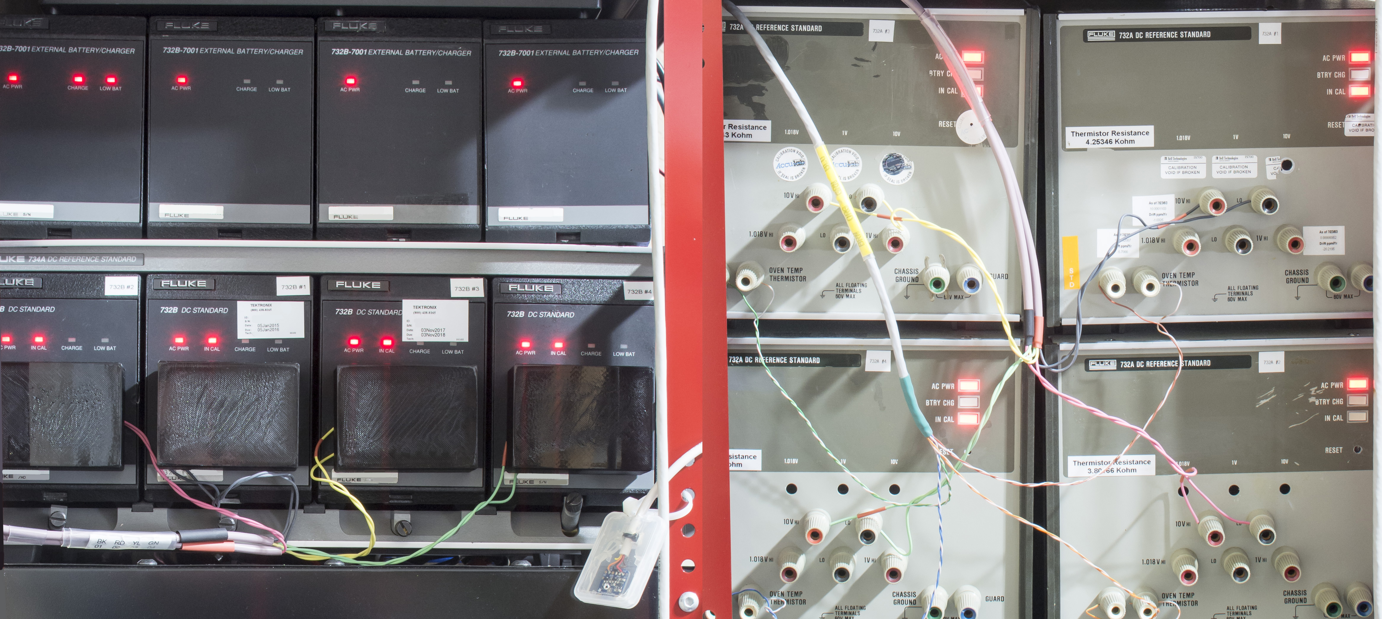
Image 12: US Lab primary DC reference bank set, 8 x Fluke 732
Main DC Voltage bank in USA consists of no less than eight LTFLU/SZA263-powered battery-backed references, running continuously and monitored with custom in-house software and Data Proof 160 + Keysight 34420A nanovoltmeter. References demonstrated stability <2 ppm a year, better than specifications.
- Wavetek 7000 (before Fluke rebranded it into Fluke 7001 DC reference, currently obsolete)

Image 13: Wavetek 7000 10V/1V travel reference cell
IET SRL-1 for 1 Ω reference point – 2 pcs, set of Fluke 742A standards
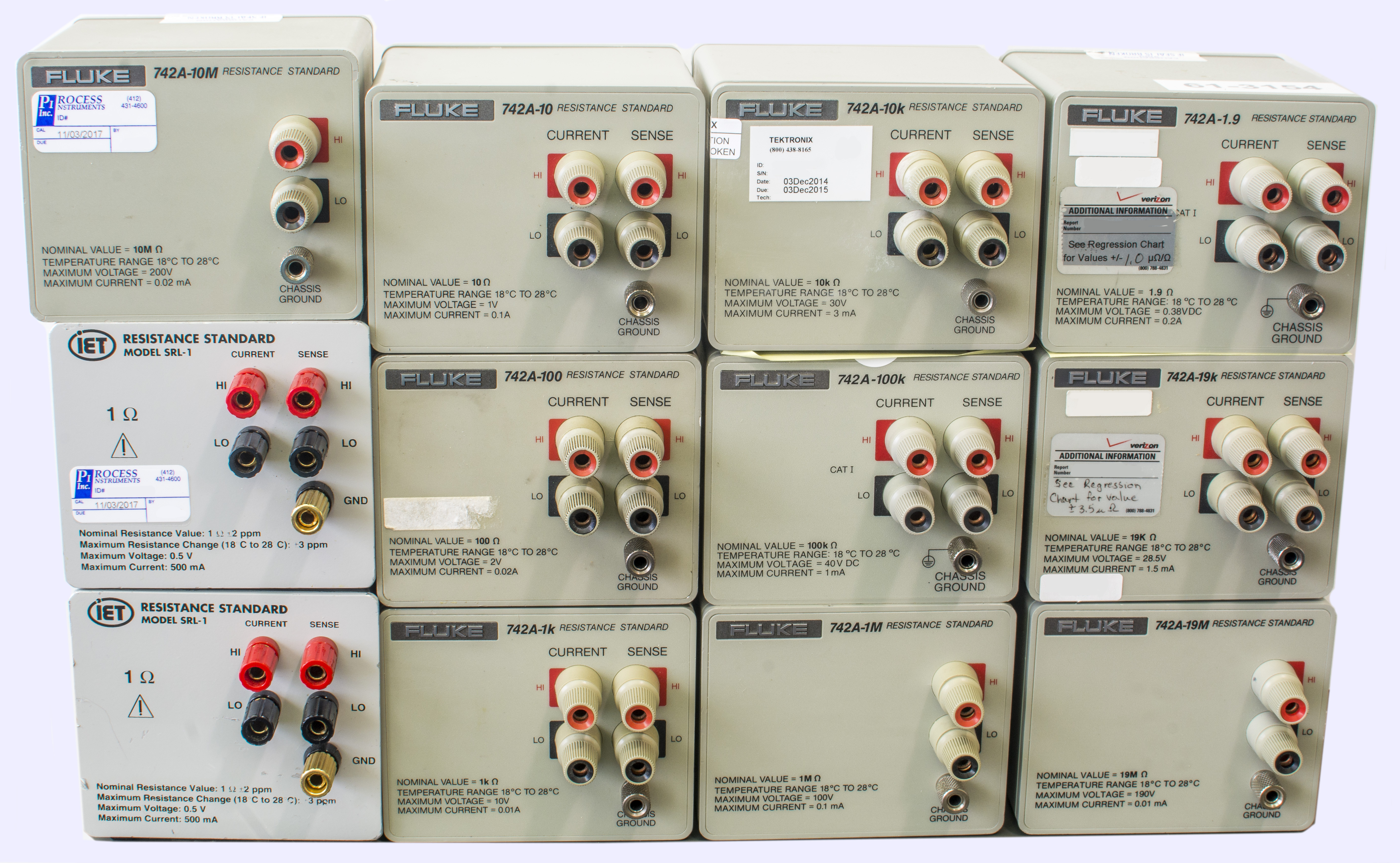

Image 14-15: Calibration resistance standards
ESI SR104 Primary Resistance Standard for 10000 Ω reference point – 2 pcs


Image 16-17: Primary 10000 Ω SR104 resistance standards
ESI 242D resistance measurement system, capable of ratiometric transfers with precision to 0.1 ppm.
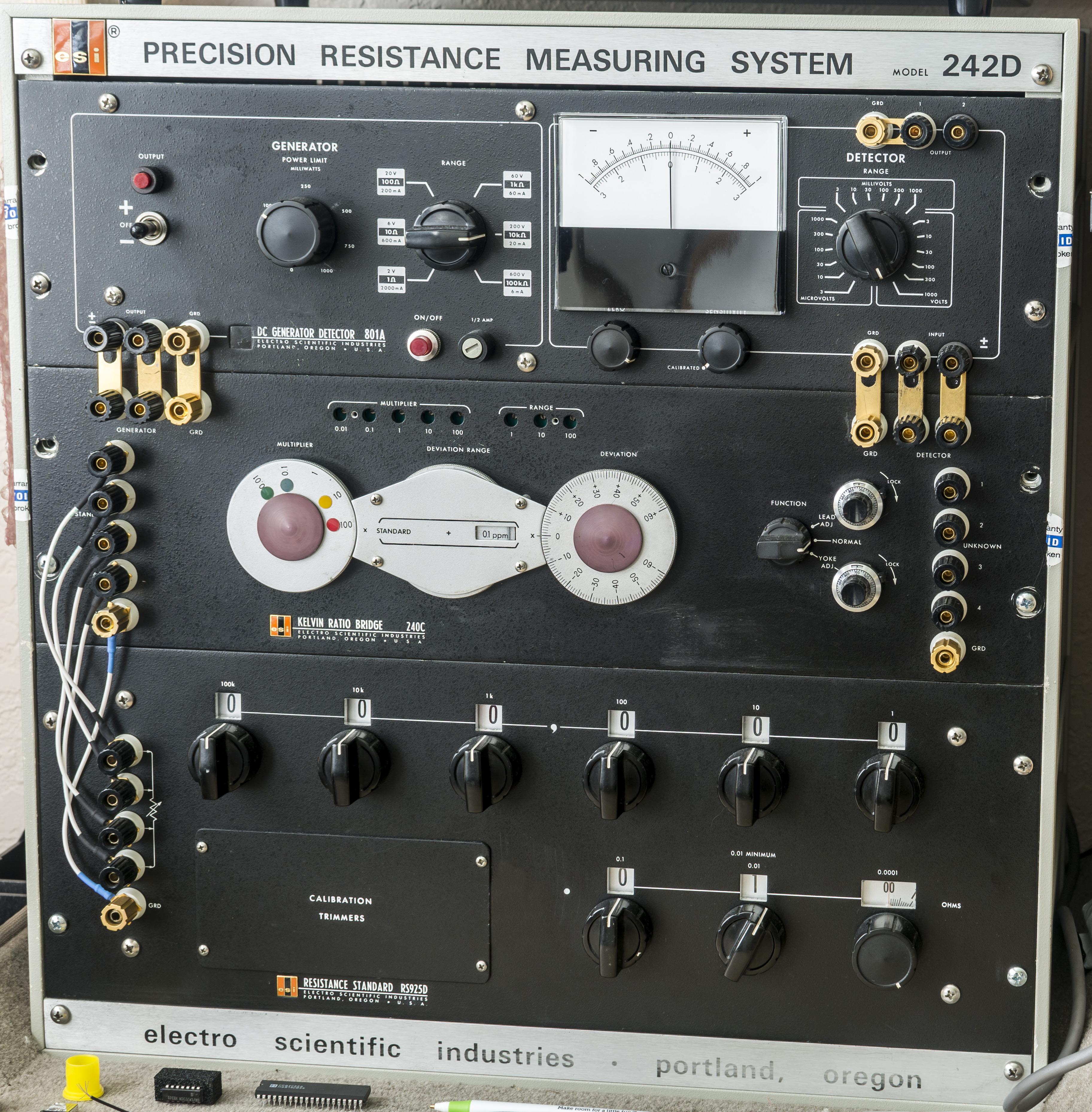
Image 18: Precision ESI 242D resistance bridge system
Agilent 3458A/001/002, calibrated by Keysight Loveland annually, check transfer standard.
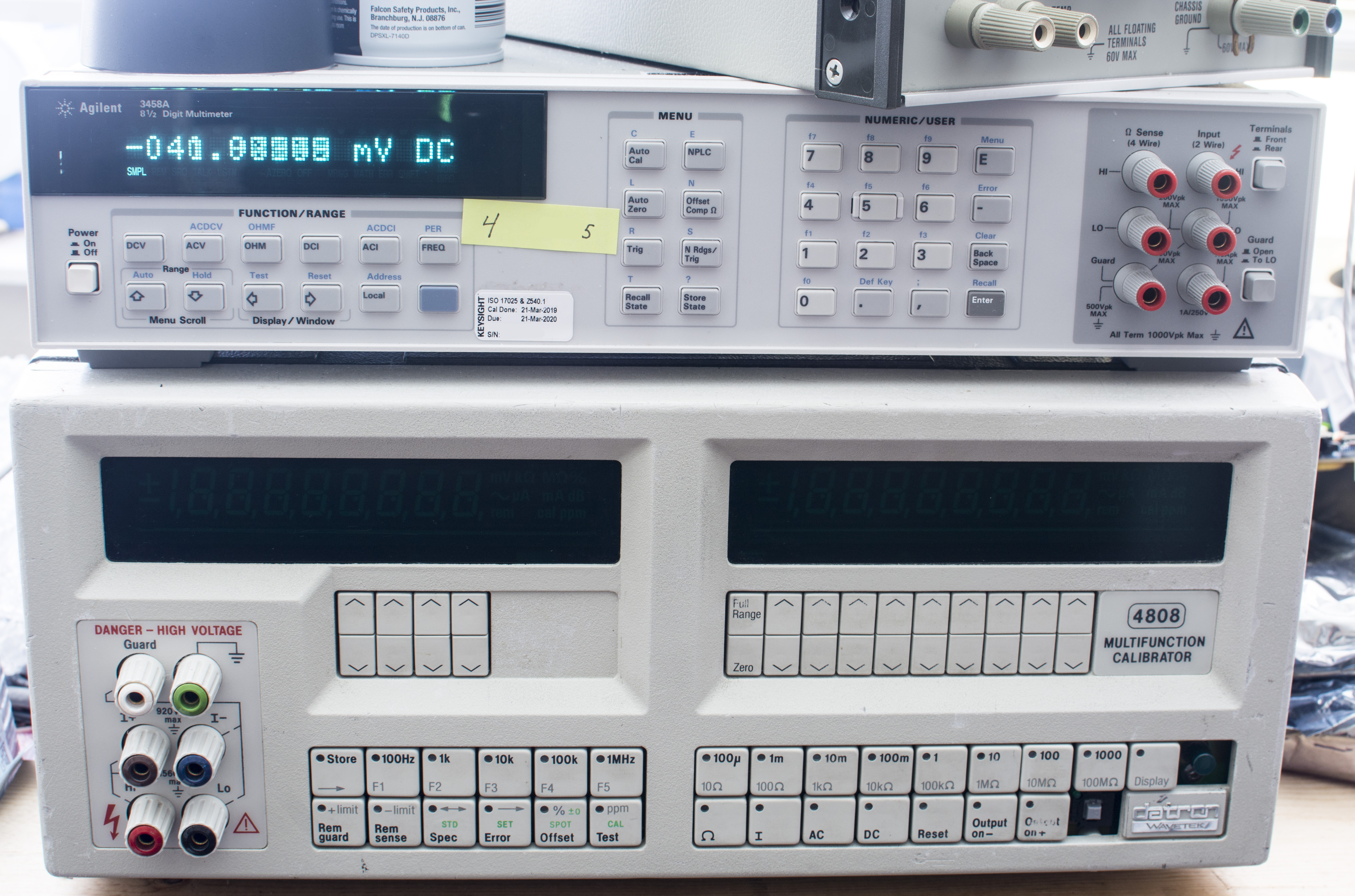
Image 19: Datron/Wavetek 4808 7½-digit MFC and Agilent 3458A/001/002 DMM
Fluke 792A AC/DC transfer standard set. It is an ultra-stable high accuracy standard, with Fluke thermal solid-state sensor. Capable to perform transfers with U < ±10 ppm and support voltage range from 2 mV to 1000V and frequency from 10 Hz to 1.2 MHz.
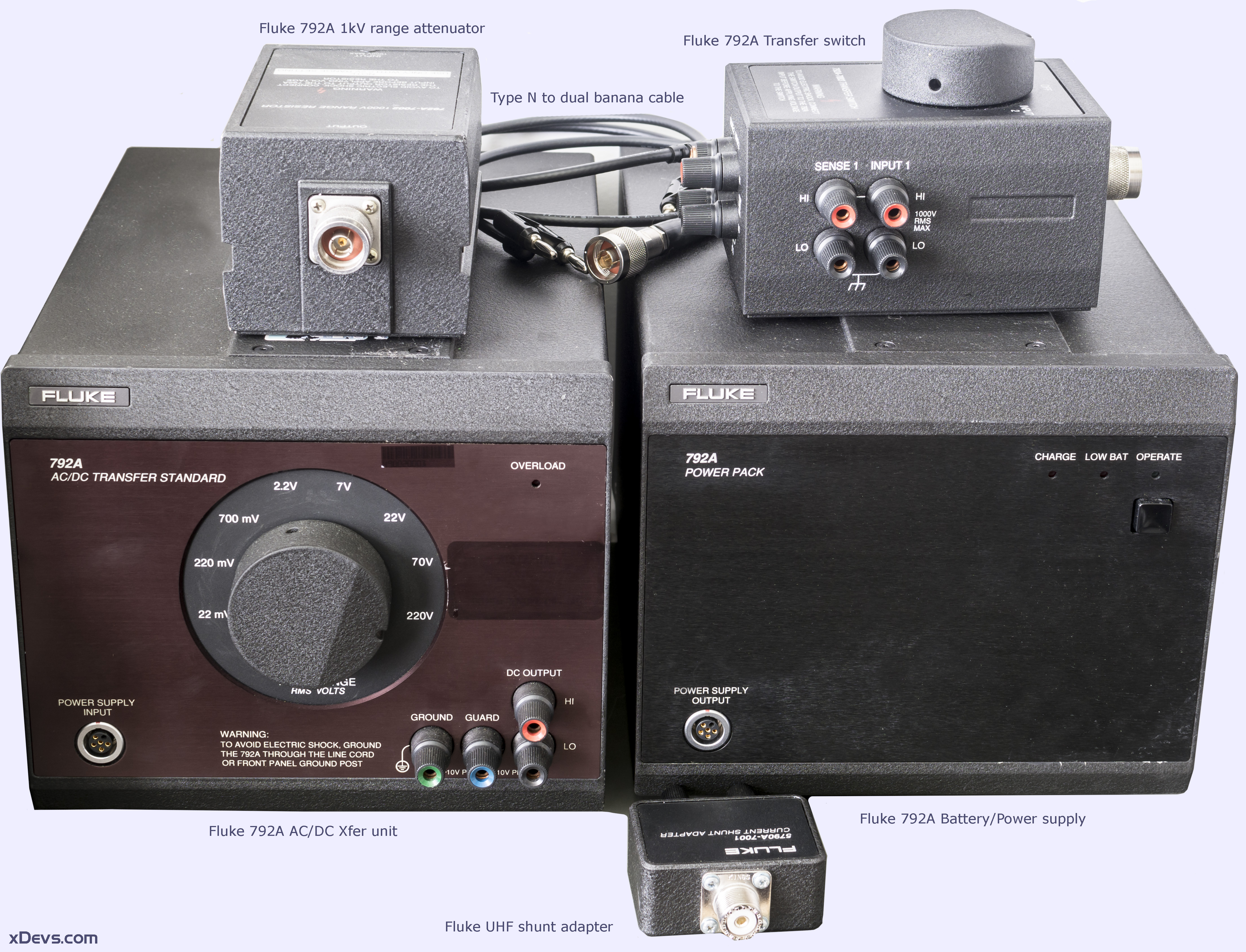
Image 20: Fluke 792A AC/DC transfer standard
Sets of various Fluke A55 Thermal Converters, Ballantine 1394N-K10 with transit cases.
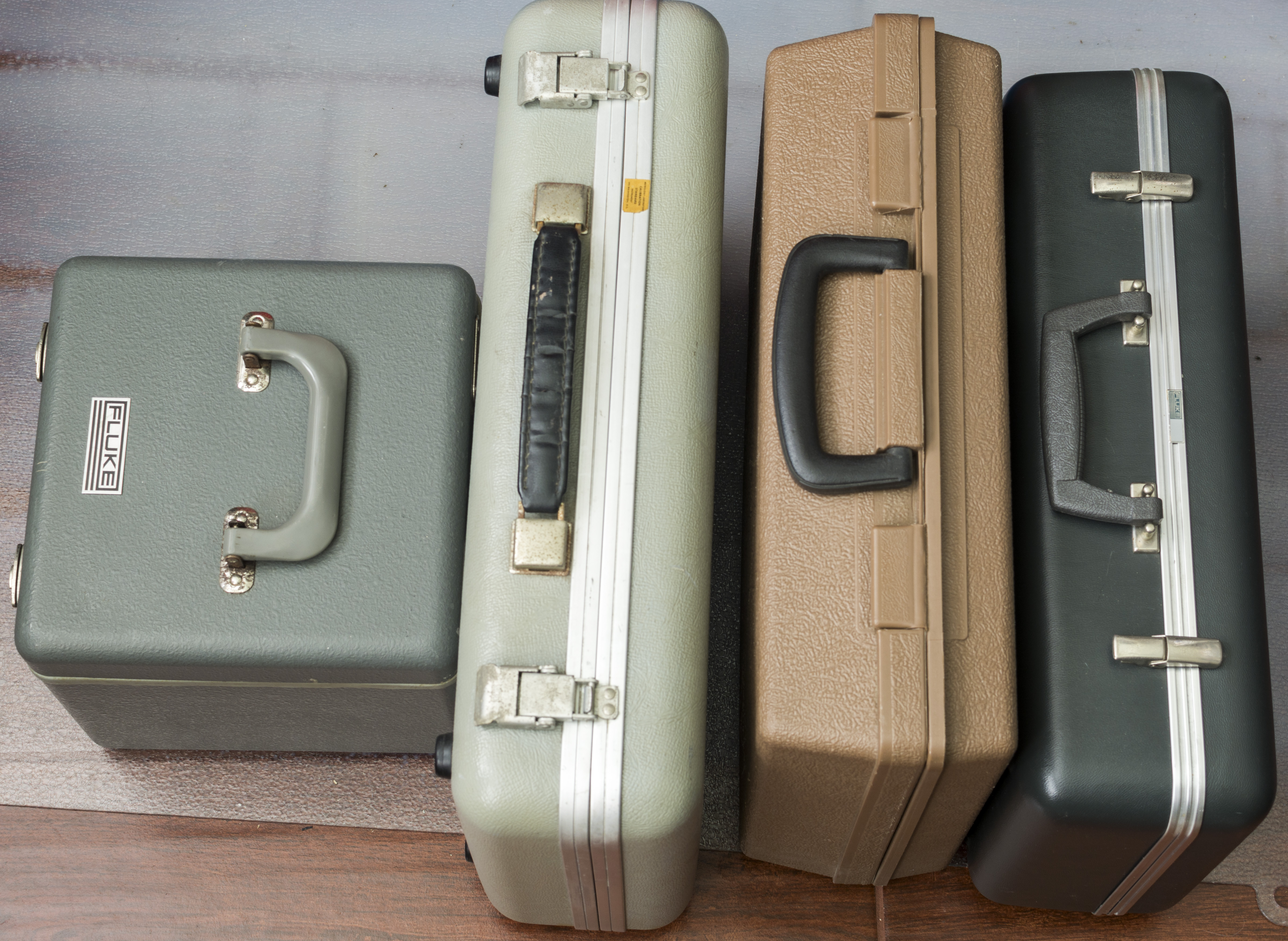
Image 21: AC Voltage thermal converters
Fluke A55’s can cover AC frequency range up to 50 MHz, at different voltage ranges. Inputs are equipped with GR-874 RF connector.

Image 22: TVC elements for various voltages from Fluke and Ballantine
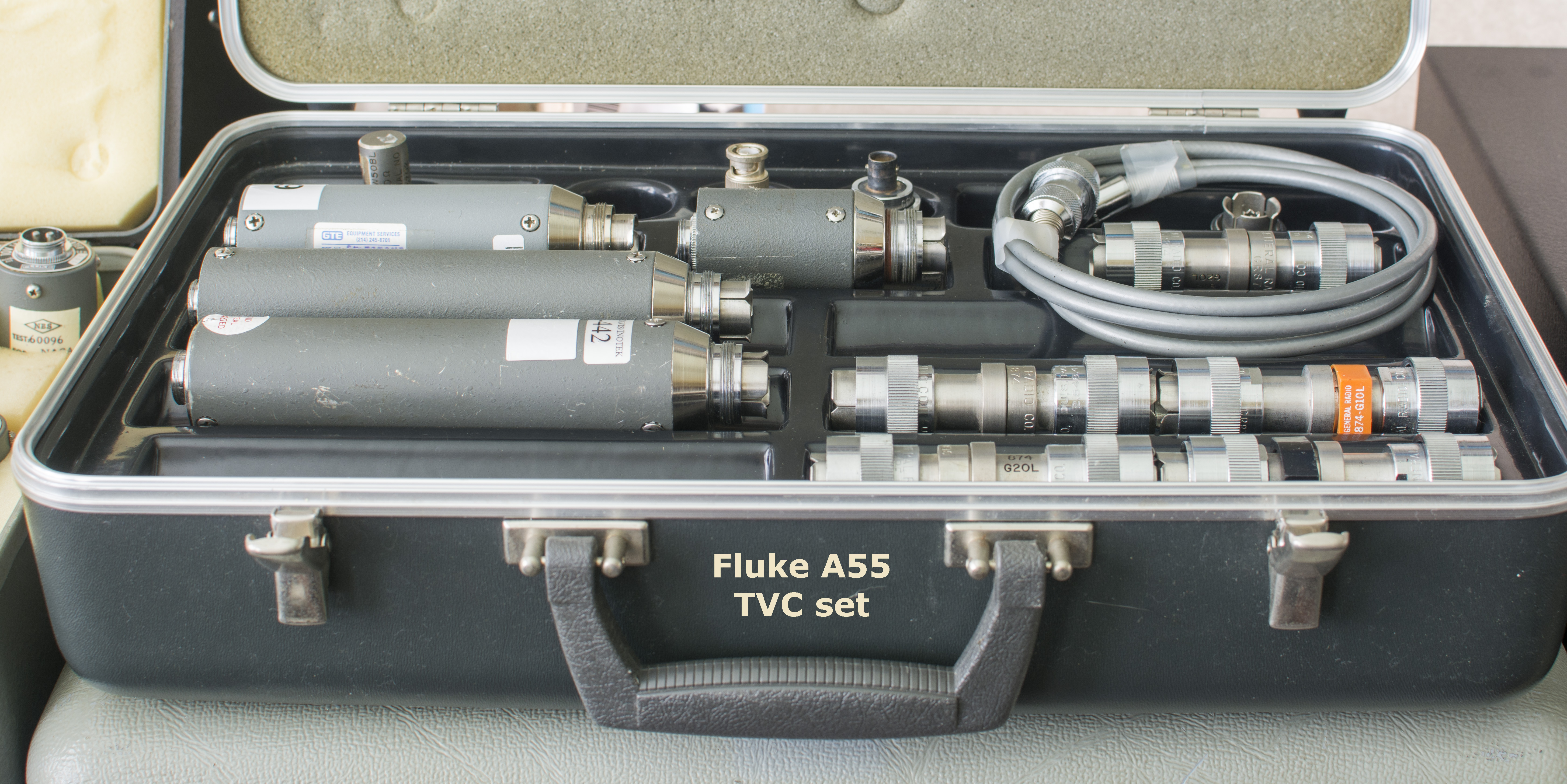
Image 23: Fluke A55 set
AC current shunt set Fluke A40A, including original case. These support AC current transfer measurements with ranges from 2.5 mA to 20 A and cover frequency between 5 Hz to 100 kHz. Typical use cases include experiments with Fluke 792A and 5700 series MFC / 5790A AVMS.

Image 24: Fluke A40 AC current shunt set
Fluke 5720A/03, 5700A/AF and Datron 4808/4800 calibrators as working standards
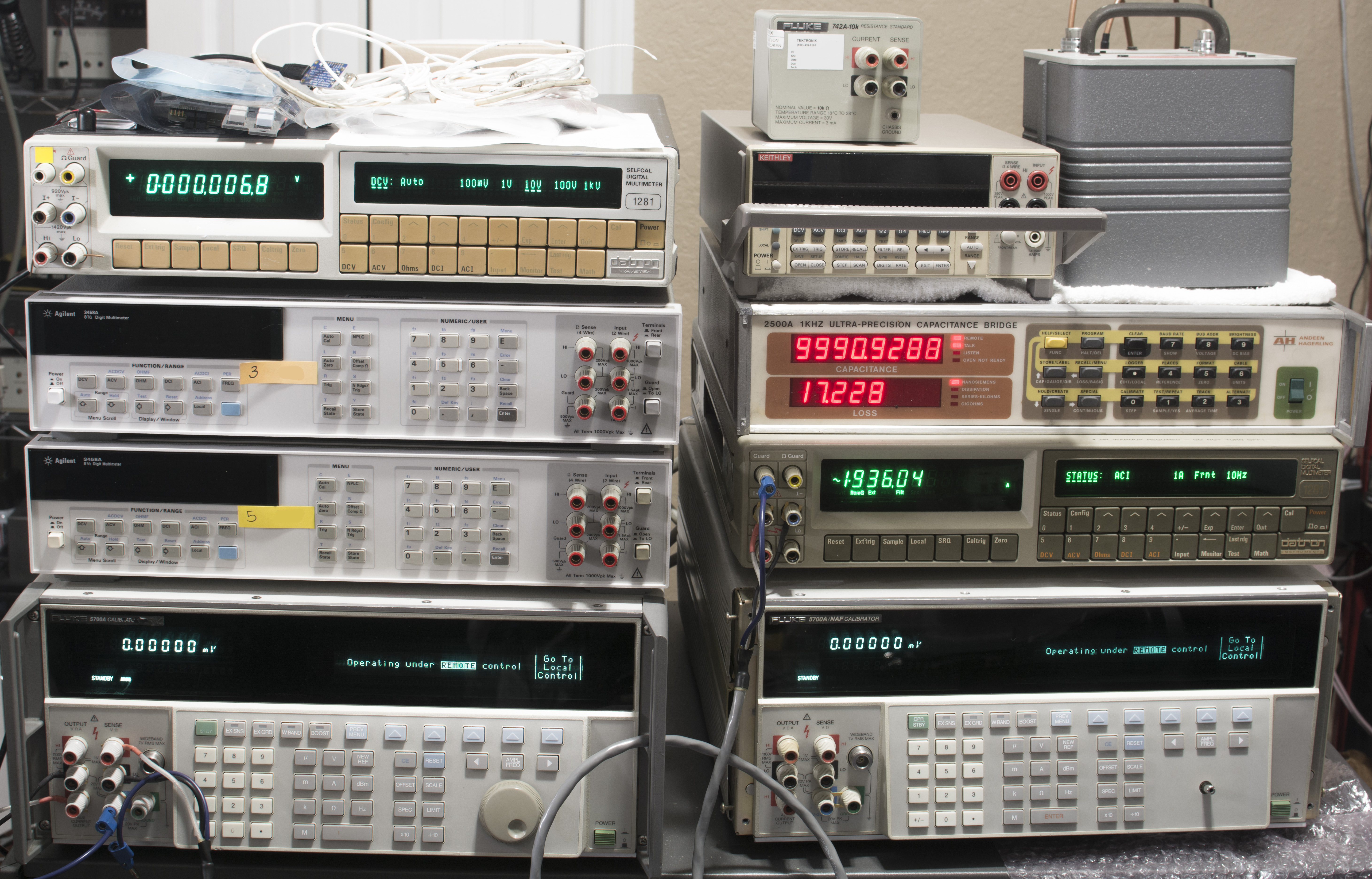
Image 25: Working standards, two Fluke 7½-digit calibrators, DMMs
Andeen Hagerling AH2500 Ultra-precision 1kHz bridge, capable measuring capacitance to 8-digit resolution with 5 ppm accuracy and annual stability less than 1 ppm. Measurement range is up to 1.2 µF.
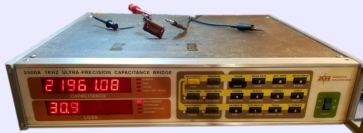
Image 26: 8 digit Ultra-precision capacitance bridge
Lab also have multiple GPSDO and Rubidium atomic frequency references, analyzers, SMUs and Keithley/Fluke/HP equipment to support various experiments.
| Function | Instrument / standard | Key specification by manufacturer | Self-calibrated instrument |
|---|---|---|---|
| Source DC Voltage, 10 V | Fluke 734A, Fluke 732A bank | ±2 ppm/year, <0.05 ppm/K TC | No |
| Source DC Voltage 1 mV – 1000 V | Fluke 5720A, Fluke 752A | ±2.5 ppm/year, relative to lab Volt | Yes |
| Source Resistance, 1 Ω | Ohm Labs 200, IET SRL-1 | ±3 ppm/year, <0.01 ppm/K TC | No |
| Source Resistance, 10 kΩ | 2xESI SR104, 742A-10k | ±0.5 ppm/year, <0.1 ppm/K TC | No |
| Source Resistance, 1 Ω – 100 MΩ | Set of Fluke 742A, 2 x Fluke 5700A, Fluke 5450A | ± <8 ppm/year | Yes (5720A) |
| Source DC Current, 100 nA – 20 A | Fluke 5700A + 5205A | ± 10 ppm/year | Yes (5700A) |
| Source AC Current, 100 µA – 20 A | Fluke 5720A + 5205A | ± 10 ppm/year | Yes (5700A) |
| Source AC Voltage, 350 µV – 1100 V | Fluke 5720A, Datron 4808 | ± 10 ppm/year | Yes |
| Measure DC Voltage, 10 V | 4 x Keysight 3458A, Keithley 2002, 2 x Datron 1281 | ± 2 ppm/year, linearity <0.05ppm | Yes (3458A) |
| Measure DC Voltage, 1 mV – 1000 V | 4 x Keysight 3458A, Keithley 2002, 2 x Datron 1281 | ± 2 ppm/year | Yes (3458A) |
| Measure DC Voltage, 10 nV – 2 mV | Keysight 3458A/Keithley 2002 + EM A10, Keithley 262 | ± 20 ppm/year, noise <0.4 nV | |
| Measure Resistance, 1 Ω – 1 GΩ | 3 x Keysight 3458A, Keithley 2002, 2 x Datron 1281 | ± 4 ppm/year | Yes (3458A) |
| Measure DC current, 100 nA – 2 A | 3 x Keysight 3458A, 2 x Keithley 2002, Datron 1281 | ± 10 ppm/year | Yes (3458A) |
| Measure AC Voltage, 10 mV – 1000 V | 3 x Keysight 3458A, 2 x Keithley 2002, Datron 1281 | ± 10 ppm/year | Yes (3458A,2002) |
| Measure AC Voltage, 250 mV – 1000 V | Fluke 792A + Datron 1281, Fluke 8920 | ± 10 ppm/year | No |
| Measure AC current, 100 nA – 2 A | 3 x Keysight 3458A, 2 x Keithley 2002, Datron 1281 | ± 10 ppm/year | Yes (3458A) |
| Compare Resistance, 1 Ω – 100 MΩ | ESI 242D and 242E, Guildline 9975, Fluke 1590 | ± 1 ppm/year | Yes |
| Measure Capacitance, 1pF – 10 µF | Andeen Hagerling AH2500 Bridge | ± 5 ppm/year | No |
| Frequency / time, 10 MHz / 1 pps | HP and Lucent Rubidium and GPSDO | ± 0.05 ppm/year | GPS |
Table 4: Key instrumentation in xDevs US Lab
Cooperation with national level metrology lab, ITRI CMS NML, Taiwan
Only xDevs’s Taiwan Lab currently participated in this SI 2019 calibration. Transfers between NML and our lab are performed by using travel artifacts, one for DC Voltage and one for Resistance. Both standards were hand-carried to metrology laboratory in Hsinchu, Taiwan to minimize transport time, reduce the chance of shipping damage and maintain less environmental stress in transit.
Dr. Shih-Fang Chen and NML team then performed measurements, using updated SI 2019 constants from their Quantum References. NML’s best uncertainty is 9.8 nV/V and 0.15 µΩ/Ω, but our final calibration result is little worse due to measurement setup and own standards instability. For those who are more familiar with typical daily life accuracy representation, this means that NML can perform calibration with error 0.0000098% for DC Voltage, 0.000015% for Resistance, which is extremely small. For comparison typical industrial digital multimeter, such as Fluke 87V have accuracy ±0.05% for DCV function or ±0.2% for Resistance (and cost also 2000 times less).
Maintaining such measurement uncertainty in any lab for the absolute unit of SI Volt and Ohm is only possible by performing periodic verification with short calibration periods. And if the transfer standard has proven and verified very good stability and performance such verification can be done in cooperation with National Measurement Lab (NML) that maintain national reference standards.
Most of the nations have their own top-level laboratory responsible for this work. Widely known national labs are NIST in USA, PTB in Germany, LNE in France. One can find more information about national labs from BIPM KCDB database
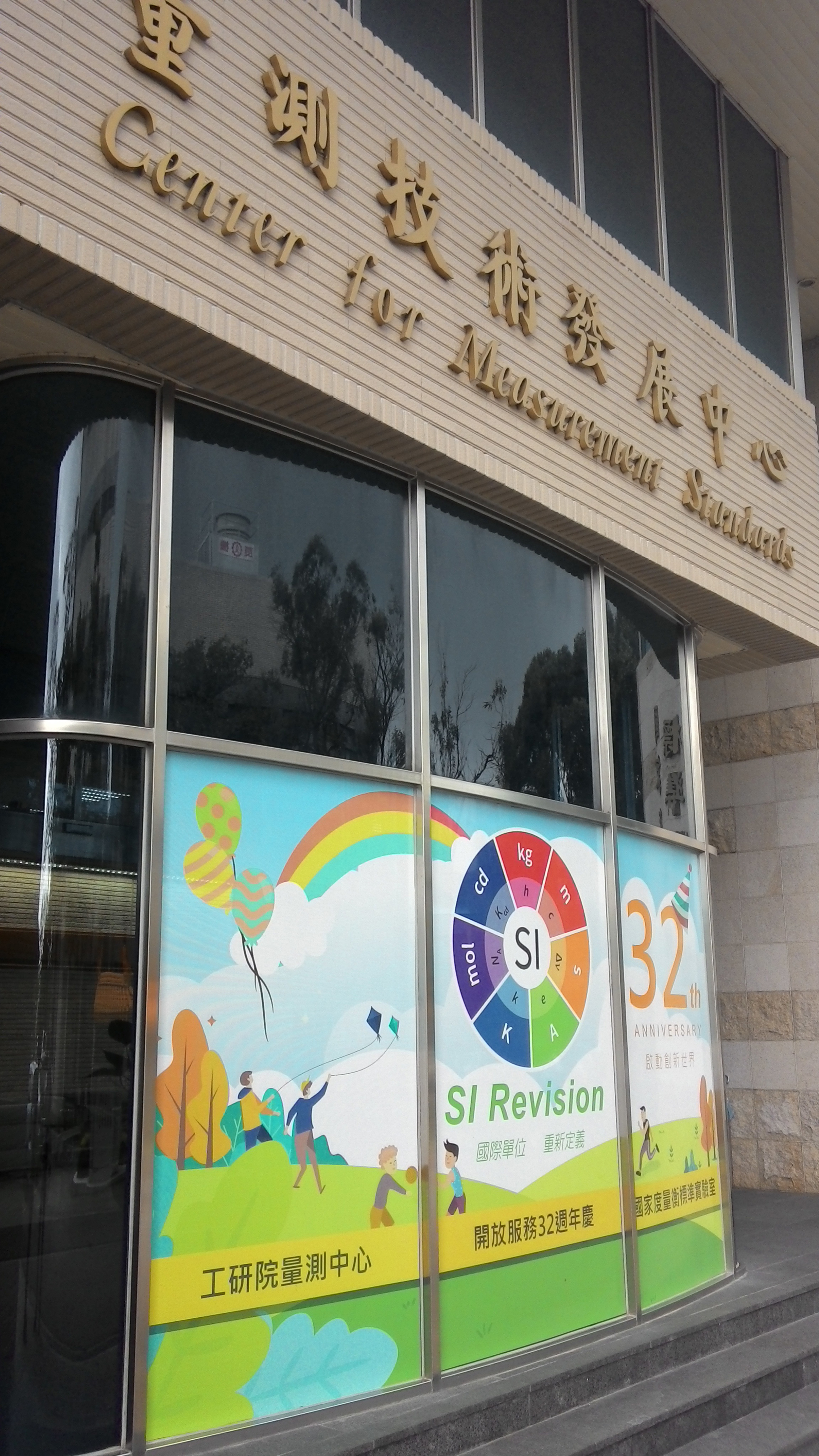
Image 27: Taiwan’s ITRI CMS National Measurements Lab Center
ITRI CMS laboratory is located in Hsinchu, the same city that have infamous TSMC fabs and also many other major semiconductor industry corporations. It was a short trip from Taipei on the High-Speed Rail (~25 minutes, $28 USD ticket) and taxi from HSR station to CMS (~20 minutes, $10 USD fare).
![]()
Image 28: Fluke 732B in Pelican 1535 Air and ESI SR104 in PC box
Standards such as Fluke 732B or ESI SR104 are reasonably robust, but it is still preferable to hand-carry fragile devices to and from the calibration facility in order to minimize possible stress and changes in output voltage/resistance. Fluke 732B was kept hot on battery backup power during transit, reconnected shortly to the AC power line to recharge upon arrival to the measurement lab. DC standard was floated on battery power again during the measurement cycle with PJVS system to avoid common-mode noise pickup from the mains power line.
Upon my arrival we proceed with a short tour, covering three main electrical laboratories.
DC Voltage Laboratory
Primary voltage standards at CMS are using Josephson effect in superconducting junctions cooled to -269 °C and secondary standards are usual room-temperature solid-state zener devices, in shape of commercial units like Fluke 732A/B and alike. Zener stability at long term is in the order of 1-5 µV/V (or 0.1-0.5 ppm for 10V output) per year.
Calibration and industry labs which using these standards must send them to primary labs for calibration measurement in every one or two years to maintain low uncertainties to few µV/V. This is required because of drift that solid-state zener sources have a predictable part (quality of the device) and a random one (stress from temperature, pressure, humidity variations, handling abuse, etc.).
Although it is possible to correct for predictable drift, the random instability has an unpredictable behavior and no mathematical models can account for that. As a result total uncertainty of uncalibrated zener reference, even if kept in safe vault still increases with time. Josephson Voltage System (JVS) is using Quantum effects to realize intrinsic, stable voltage output. This is the main reason why JVS standards are used by national level metrology organization like CMS, enabling international maintenance of SI Volt and calibration services to customers with solid-state zener references.
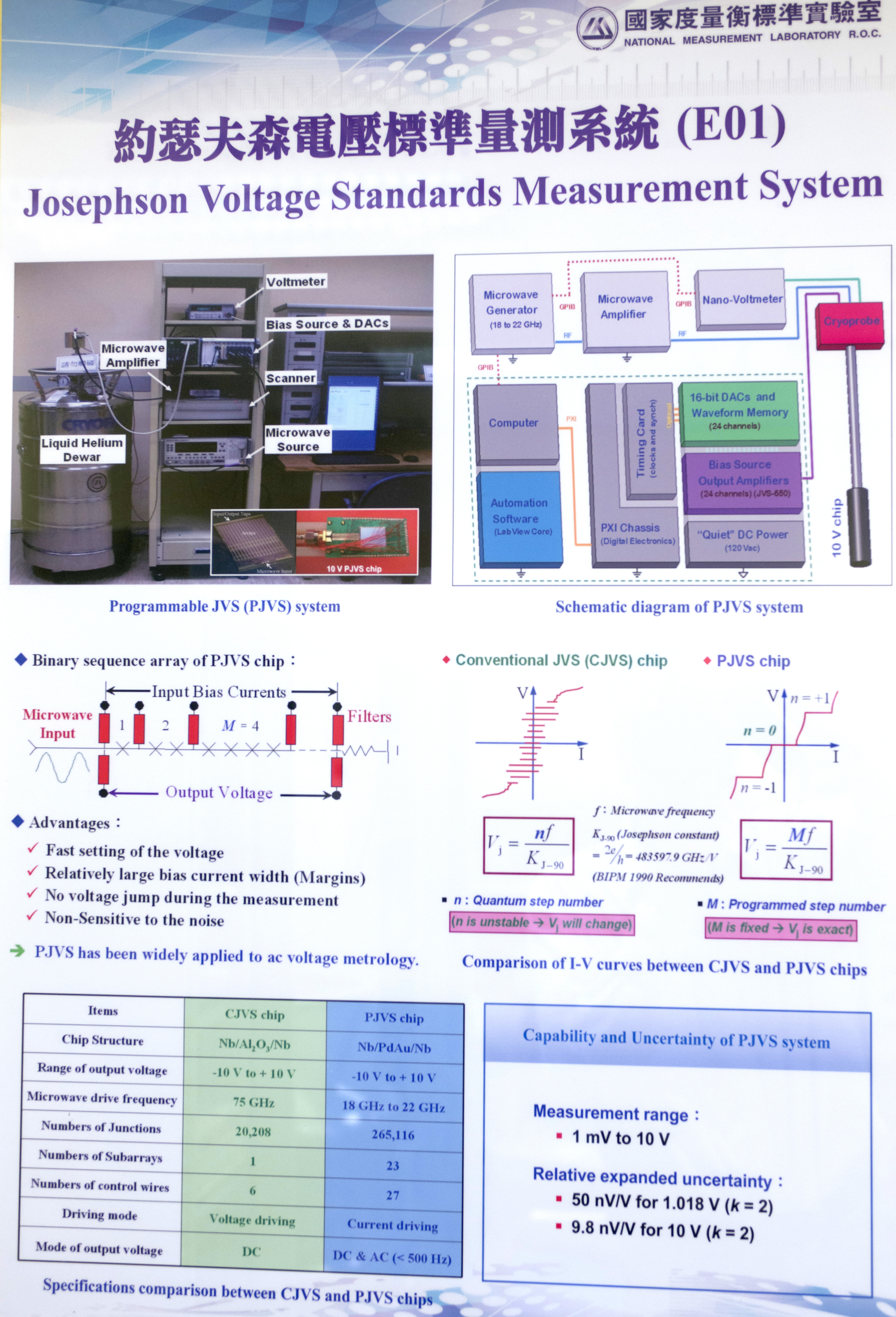
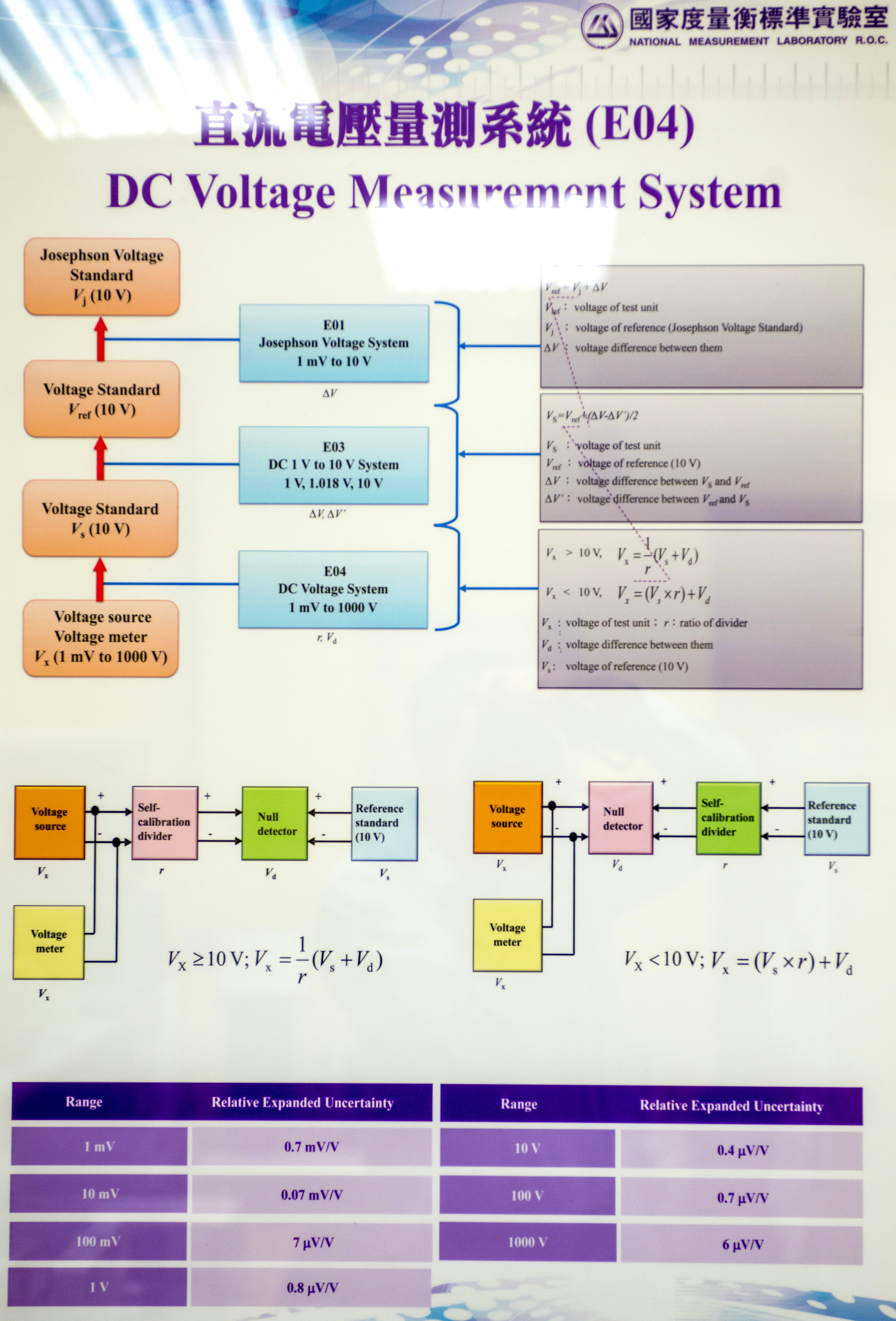
Image 29-30: DC Voltage Lab posters
A large poster on the wall highlights the key difference between conventional JVS (CJVS) and programmable (PJVS). CJVS use high-frequency RF and voltage bias to produce fixed voltage steps, while PJVS using lower RF input with multichannel current bias, also able to produce AC signals with low frequency.
The voltage output generated by Josephson chip is by definition exactly equal nƒ/KJ but in actual measurement setup there are always errors, induced by RF frequency instability, the noise of the null detectors, switch EMF, cable leakage and resistive loss, EMI interference, junction defects, bias currents. Major error sources that contribute to transfer uncertainty are DUT’s zener reference noise and switch thermal EMF offsets, resulting in uncertainty specification assigned to JVS calibration.
Some of these errors can be measured and corrected, some others cannot be predicted, DUT noise or drift stability. Typically, the total uncertainty contribution of a JVS source itself includes multiple readings taken during the calibration method and have a level just within few nanovolts. That is a tiny fraction of own 732B’s typical noise specification 680 nV (SDEV from 10V output regression).
Taiwan’s CMS has four types of calibration service for DC Voltage. The top tier is solid-state reference calibration E01, directly against cryocooled NIST PJVS system. This is the most expensive calibration, with the lowest uncertainty available. Voltage levels of DUT standards must be in a range from 1 mV to 10V, to obtain best transfer accuracy from the array. This is the service that we have chosen for Fluke 732B calibration.
| CMS calibration tier | E01 | E03 | E04 | E05 |
|---|---|---|---|---|
| Reference | Quantum NIST PJVS | Bank of Fluke 732 | MFC + Divider setup | HV setup |
| Calibration DUT voltage | 1 mV – 10 V | 1 V, 1.018 V, 10 V | 1 mV – 1000 V | 1 kV – 200 kV |
| Uncertainty | 0.05-0.1 µV/V | ~0.3 µV/V | 6 – 700 µV/V | 100 µV/V |
| Estimated price | $580 USD | $345 USD | $210 USD | $210 USD |
Table 5: DC Voltage calibration services from ITRI CMS (June 2019)
Taiwan’s National Volt also has secondary solid-state reference ensemble, in form of six stand-alone Fluke 732B. Three of them were specially modified by Fluke to provide cardinal point 1.0000 VDC instead of standard 1.018 VDC. 1.018638 V level was used back in the days before 1990. This voltage was the output of the Weston-type chemical cells, that used provided International Standard for EMF from 1911 till retirement from Josephson systems in 1990.
Weston cells are still used today in metrology, despite being very fragile, incapable to sustain any current draw and difficult to maintain. Weston Cells also imply significant HazMat risk, due to a significant amount of cadmium, mercury, and related toxic chemicals. The groups of well-maintained Weston Standard Cells highly stable over time otherwise, but they are more often replaced with zener diode solid-state DC voltage standards, which are more robust and convenient to use. The output of solid-state reference, however, drifts with time and is also subject to environmental conditions changes like ambient temperature, relative humidity, and pressure. To obtain the best accuracy it is necessary to construct a mathematical model of the particular reference device to predict its output voltage at any given time and under given environmental conditions.

Image 31: National Volt, six Fluke 732B solid-state reference bank
Commercial solid-state references are based on only one high quality selected zener devices such as Linear LTZ1000/LTZ1000A, Linear LTFLU-1 or older Motorola SZA263. Use of since chip making it impossible to detect any variation of this critical component without external stable and known reference.
Most labs as a result use multiple units of solid-state references, to form a multi-device bank for reducing the variation of the averaged “Lab’s Volt”, and to detect variations between individual devices. Such a system, when monitored periodically can also help to detect damaged units which may have excessive drift or sudden output voltage jumps. xDevs.com labs also follow this idea, and we use both multiple solid-state zener devices to keep “xDevs.com Volt” together with multiple detectors (Keysight 3458A and Keithley 2002). Adding meters into the validation loop also helps to cover the stability of LTZ1000 references used in these high-end DMMs.
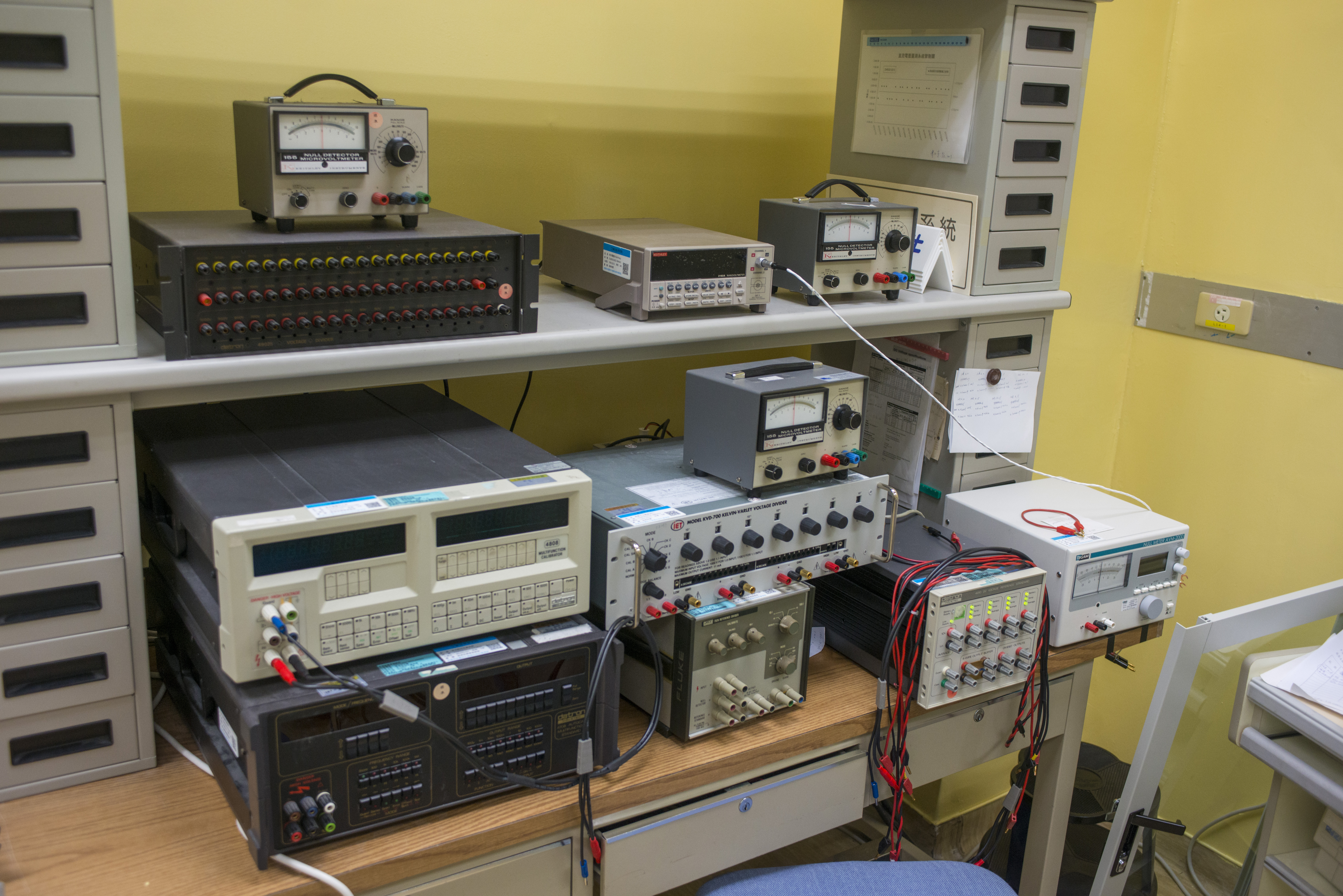
Image 32: Dividers, calibrators, nanovoltmeters and more DC references
Set of dividers and high-end calibrators are used for E04 service, when customers need calibration of their dividers or measurement/source instruments, such as calibrators, DMMs or sources. We can see good old Datron 4708, Datron 4808, set of very nice Keithley 155 null-meters, special and rare Datron 4902S filled with hundreds of metal foil VHP resistors, IET KVD-700 0.1 ppm manual divider. There is also Fluke 752A reference divider, Datron 4910 with 4 LTZ1000A-based cells and Keithley 2182A nanovoltmeter.
Lab is currently testing new binary voltage divider, manufactured by Measurements International, Model 8000B.
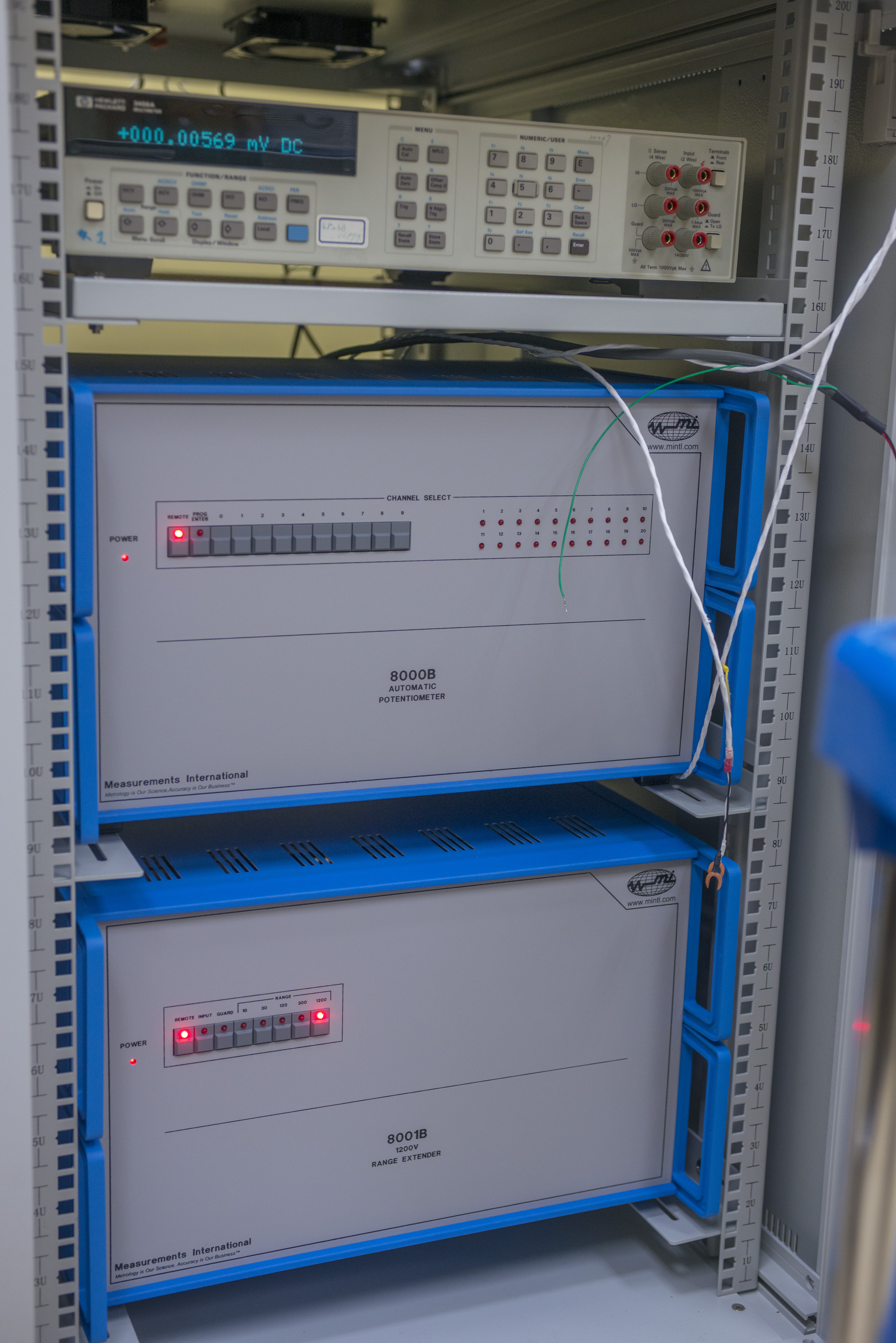
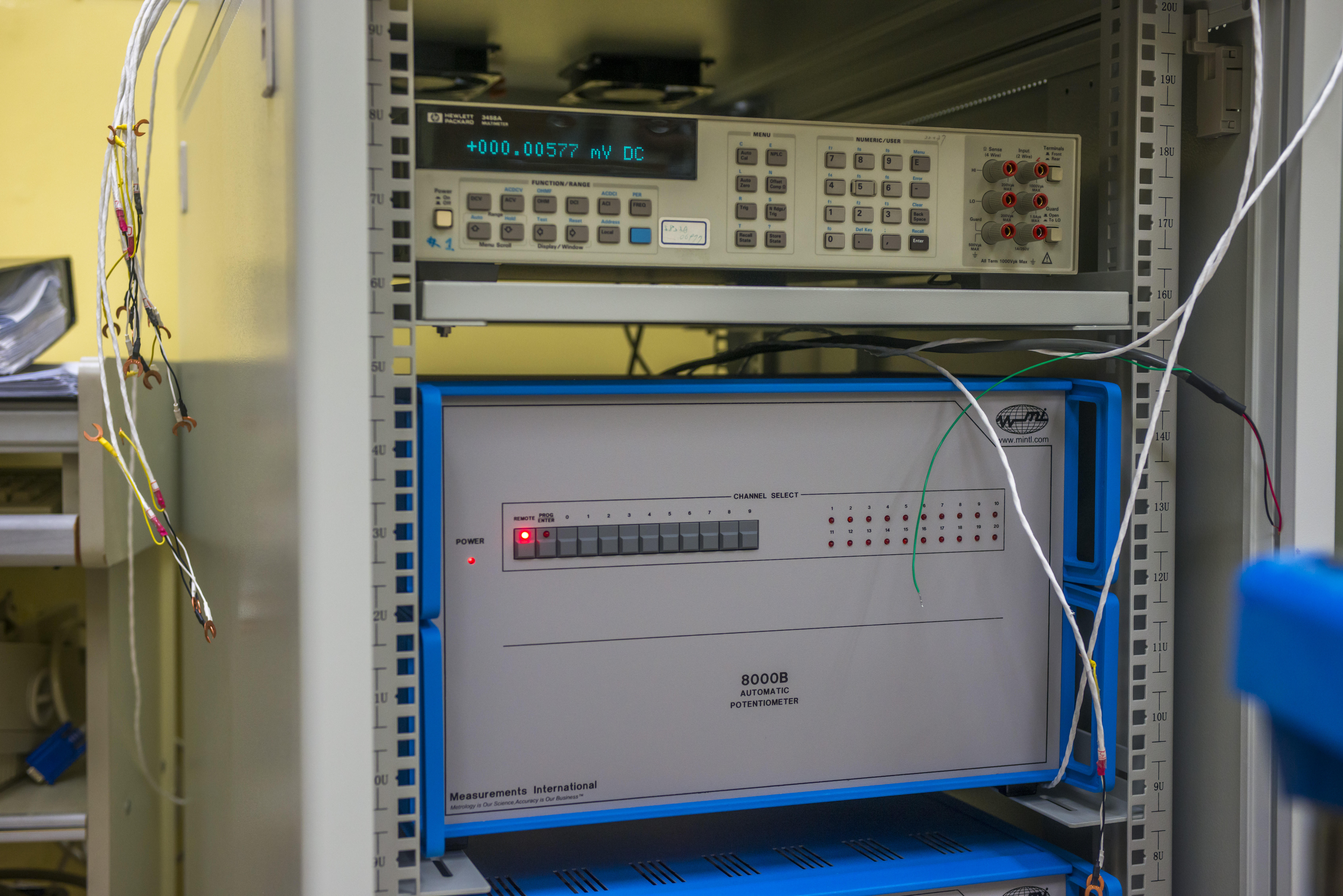
Image 33-34: New ultra-linear binary divider setup, Measurements International 8000B
MI 8000B is modern replacement of hard to find Fluke 720A, providing arbitrary very accurate output voltages with linearity better than 0.02 ppm. Its nominal resistance is 1.2 MΩ and setting resolution is 9 digits.

Image 35: Solid-state zener transfer check using Dataproof scanner and 3458A
Clock reference for the system is an atomic frequency standard using rubidium atom transition frequency to discipline output XO. It is implemented by Symmetricom (today Microsemi) 8040, mounted on the CJVS rack. HP 53132A counter monitors frequency output for control.
Quantum Voltage standard, NIST SRI 6000q
SI Volt at CMS is provided by NIST SRI 6000q PJVS. This PJVS can generate stable, quantum-accurate, DC voltages, programmable in the range from -10 volts to +10 volts.
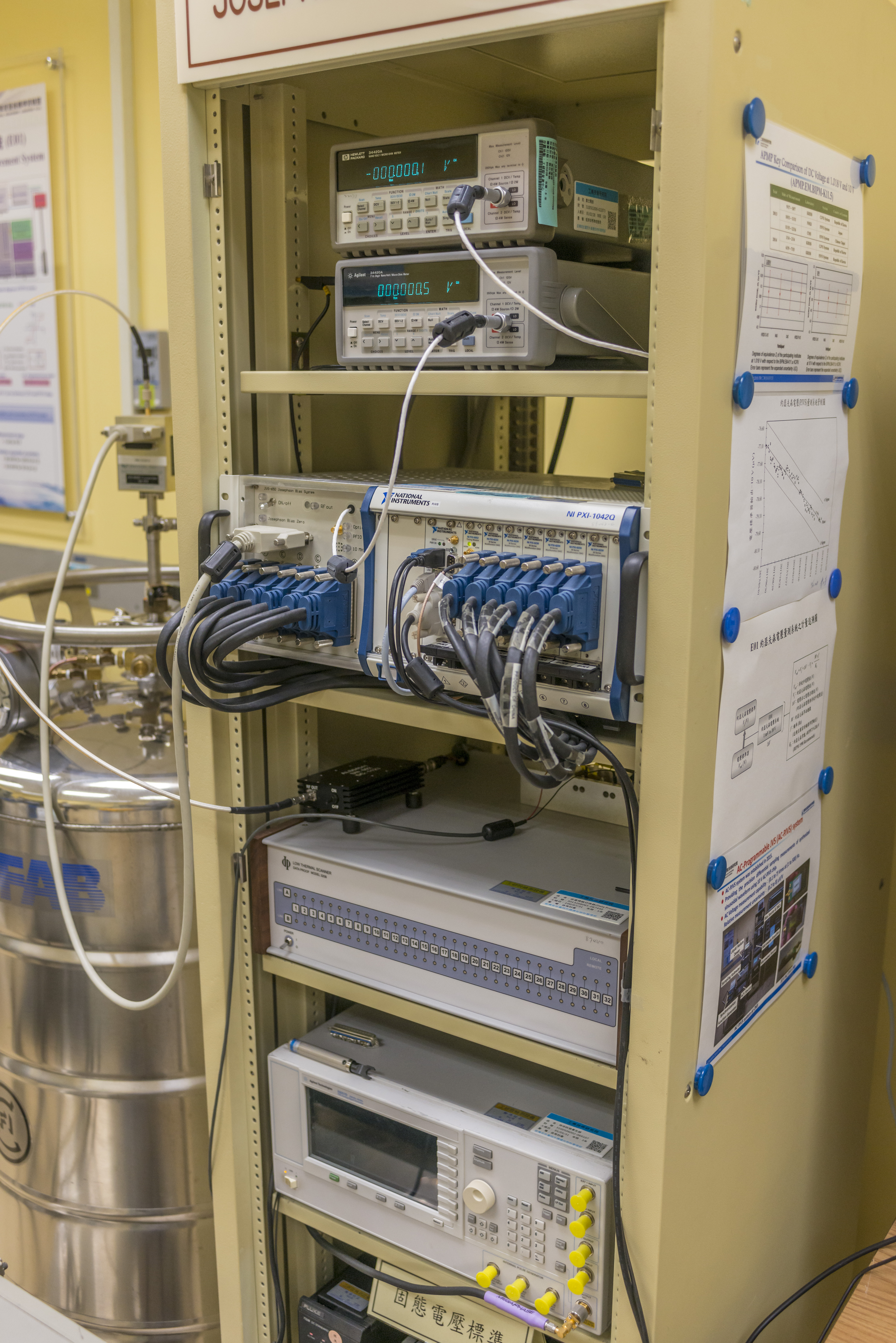
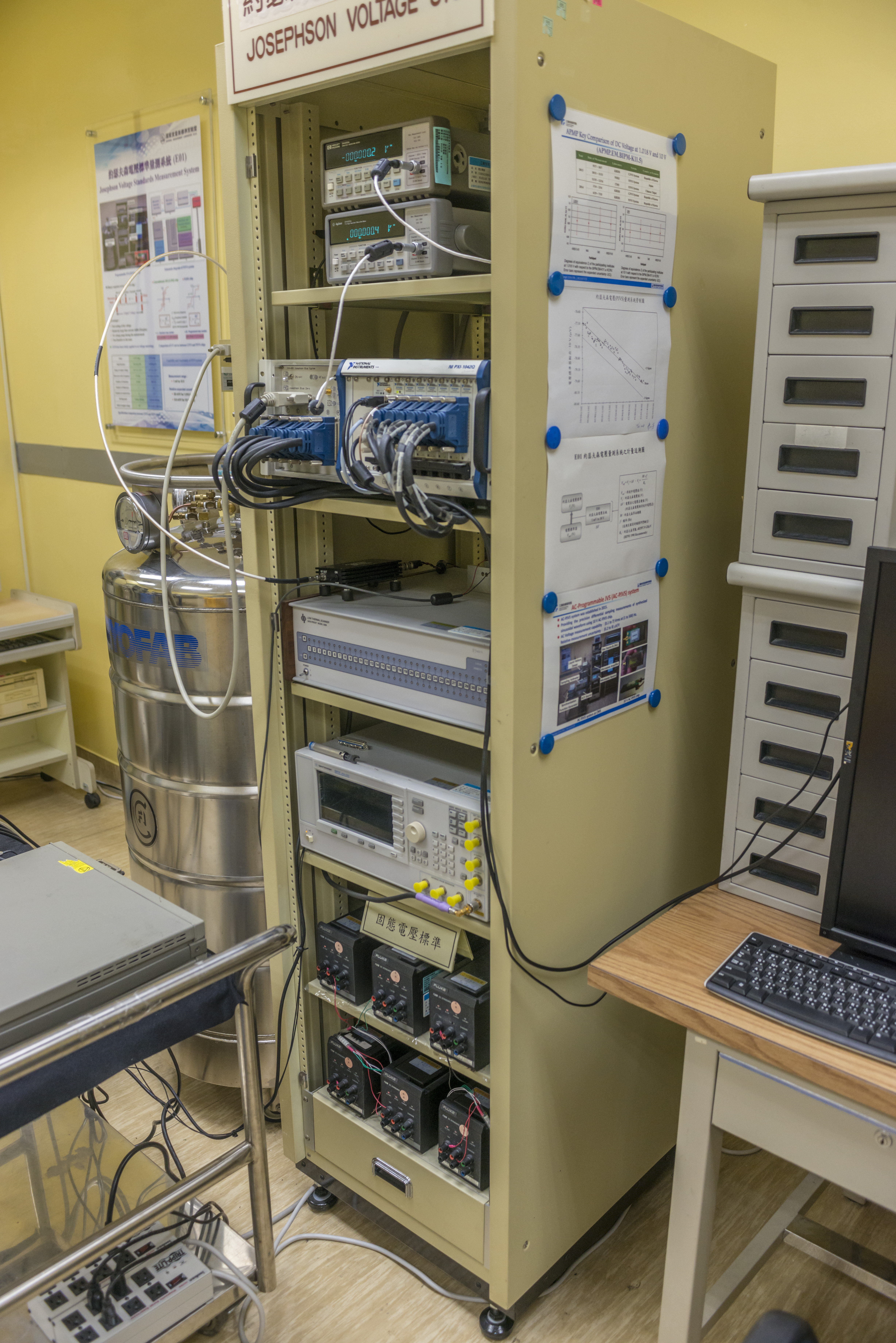
Image 36-37: NIST SRI 6000q PJVS at ITRI CMS National Lab in Taiwan
The quantum accuracy of these voltages is derived from the Josephson Effect such that every superconducting Josephson junction in the PJVS circuit produces a voltage precisely proportional to the frequency of the applied microwave bias signal.
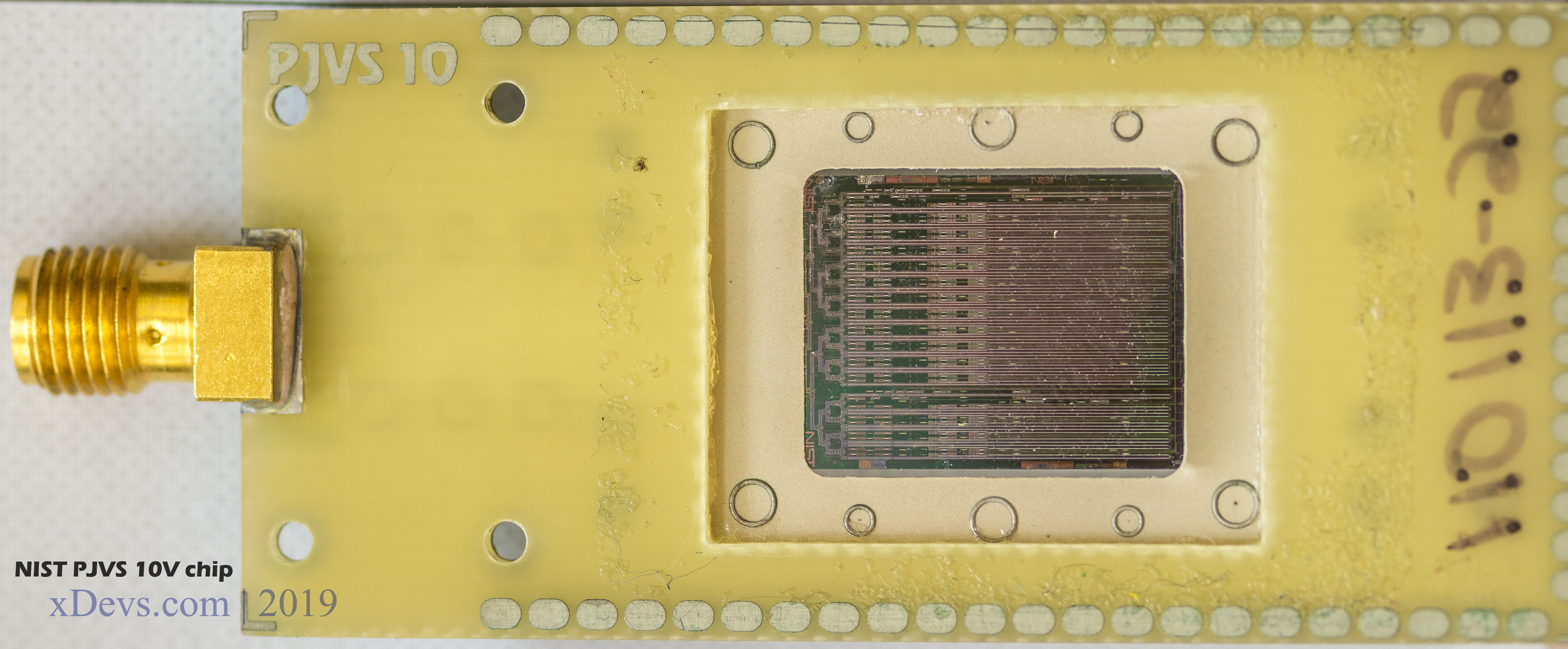
Image 38a: NIST PJVS 10V chip superconductor junction arrays structure, active side
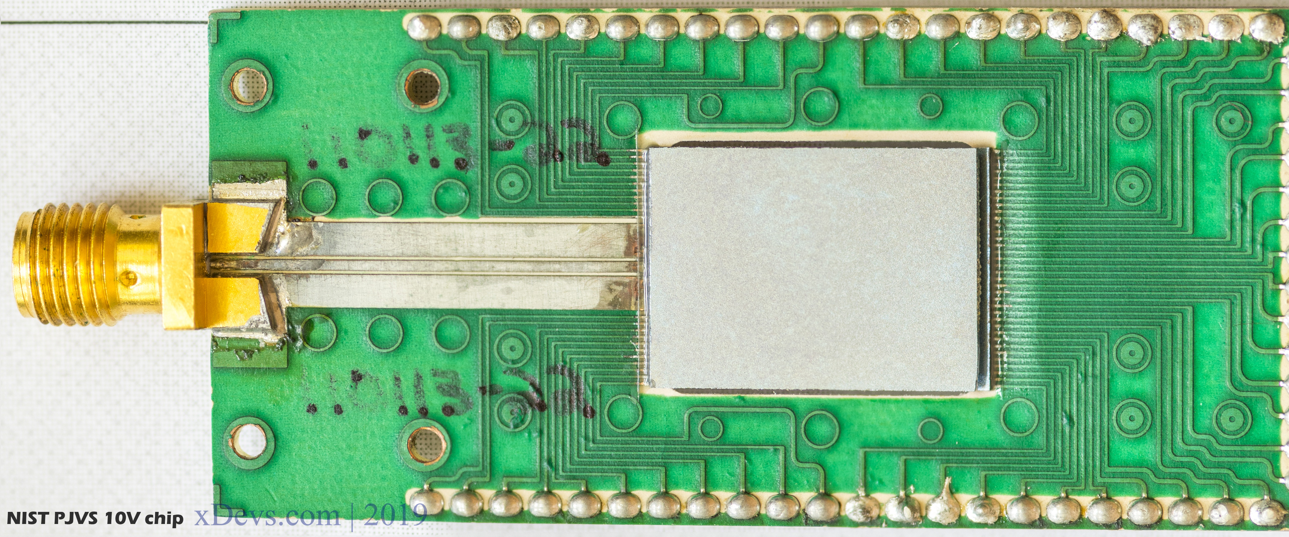
Image 38b: NIST PJVS 10V chip carrier (this sample on the photo is damaged)
Image 38 shows NIST 10V PJVS assembly with wire-bonded chip package on RO4003C dielectric top layer PCB. This particular package has SnPb plated traces, except in the locations where the wire bonds connect.
Cryoprobe is the physical interface between a Josephson voltage standard (JVS) chip and its RF and bias electronics system. The cryoprobe is compatible with standard liquid helium Dewars and provides a gas-tight and RF tight seal at the top of the Dewar flange. Operating frequency for PJVS array is in the range 18 GHz – 22 GHz, so this system does not need high-frequency source like older ones.
Complete reference system consists of next hardware:
- HPD JVS-650B cryoprobe
- HPD JVS bias interfacing box
- Cryopackaged NIST 10V PJVS superconductor chip
- Cryofab CMSH-100 Dewar with fixtures compatible with HPD JVS cryoprobe
- Agilent E8257D-528 microwave synthesizer with frequency up to 31.8 GHz
- Aldetec ALS04541 microwave amplifier
- Agilent/Keysight 34420A nanovoltmeter
- National Instruments PXI-1042Q chassis, PXI-8101 controller, 6 x PXI-6230 DAC cards, 6 x DB37M-DB37F-EP 37-Pin Shielded Cables, PXI-6652 Timing module.
- GPIB cables, auxiliary cables to nanovoltmeters, etc.
- NISTVolt “ZenerCal, DVMcal and PJVS-Core” system software
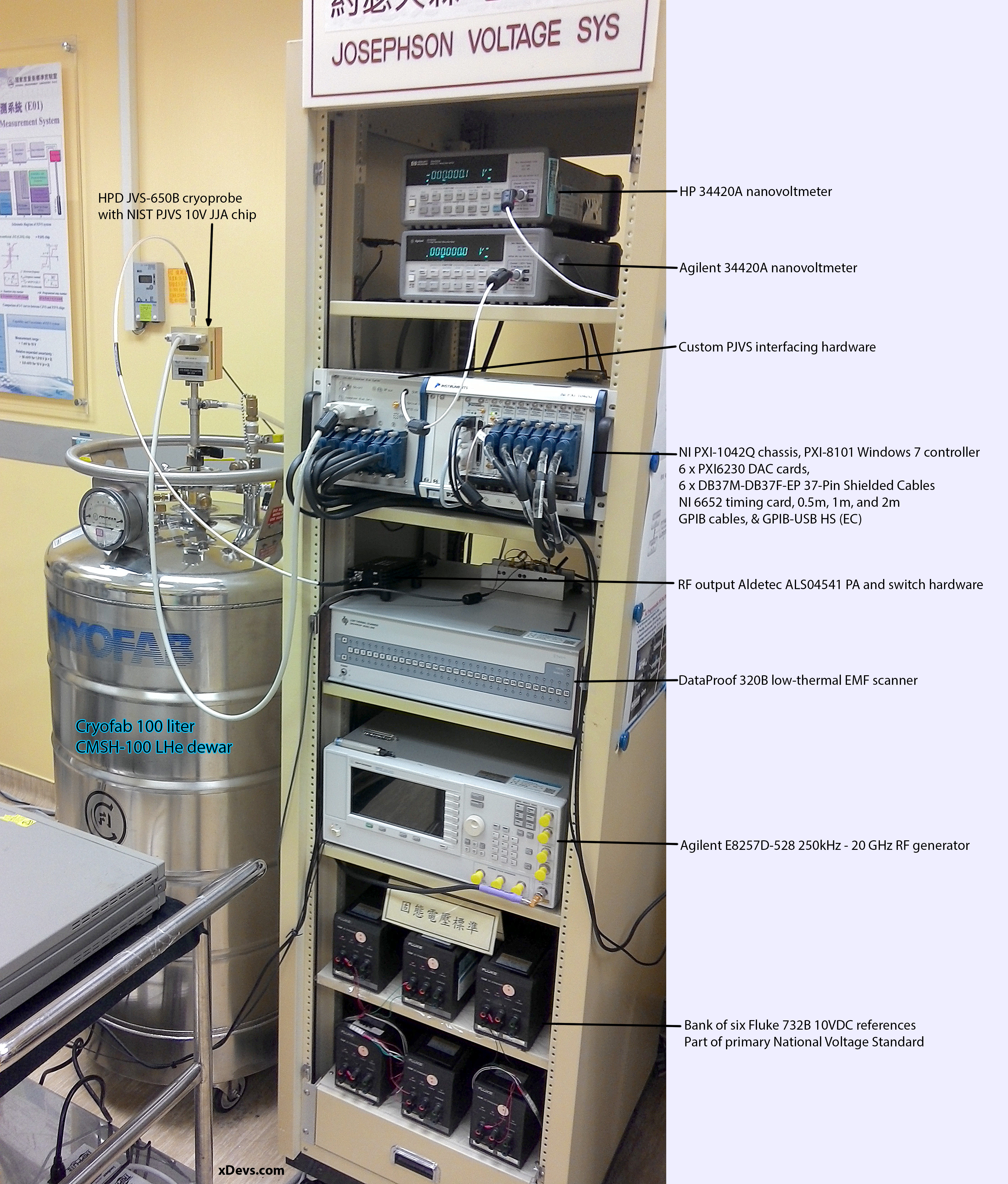
Image 38: System breakdown with notes on each item
Nearly all hardware is commercially available. The only special parts are cryoprobe with NIST superconducting chip with Josephson array, RF microwave amplifier, bias interface and NIST control software. This makes system expensive, but serviceable in short time if RF source, detector or PXI module develop a failure.
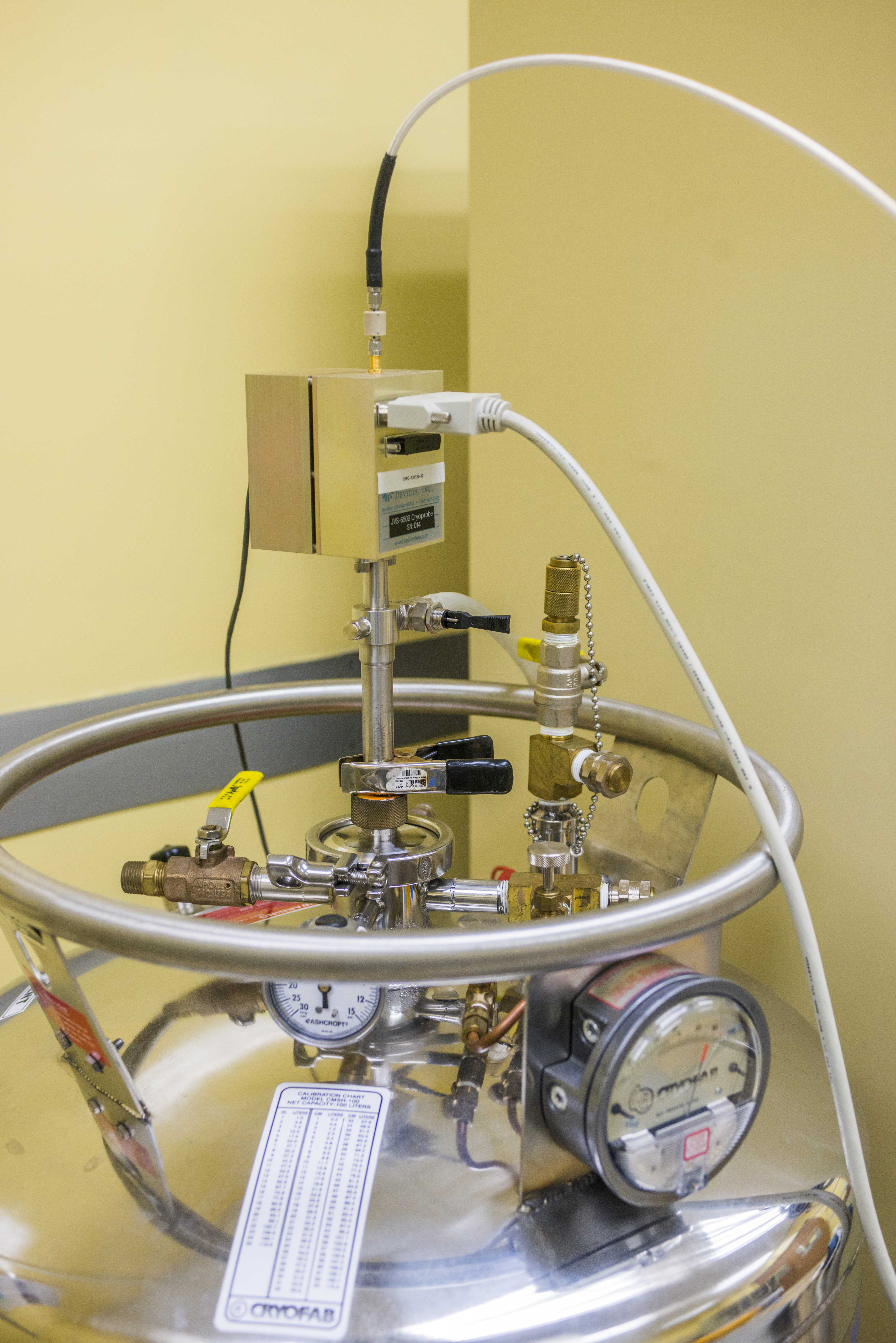

Image 39-40: NIST PJVS system cooling tank and cryoprobe interface
Because Niobium junctions on Josephson Array chip can become superconductive only at a temperature below 5K (-268.15 °C) Liquid Helium is required to provide cooling. That is what large 100-liter tank from Cryofab contain when the system is in active operation. That amount of helium is evaporated by a period of three weeks, resulting hefty price to keep in JVS apparatus in operation. Many labs do not keep JVS operating all the time, but only use them on cycle periods during few months to perform calibrations and transfers of quantum Volt to solid-state reference array.
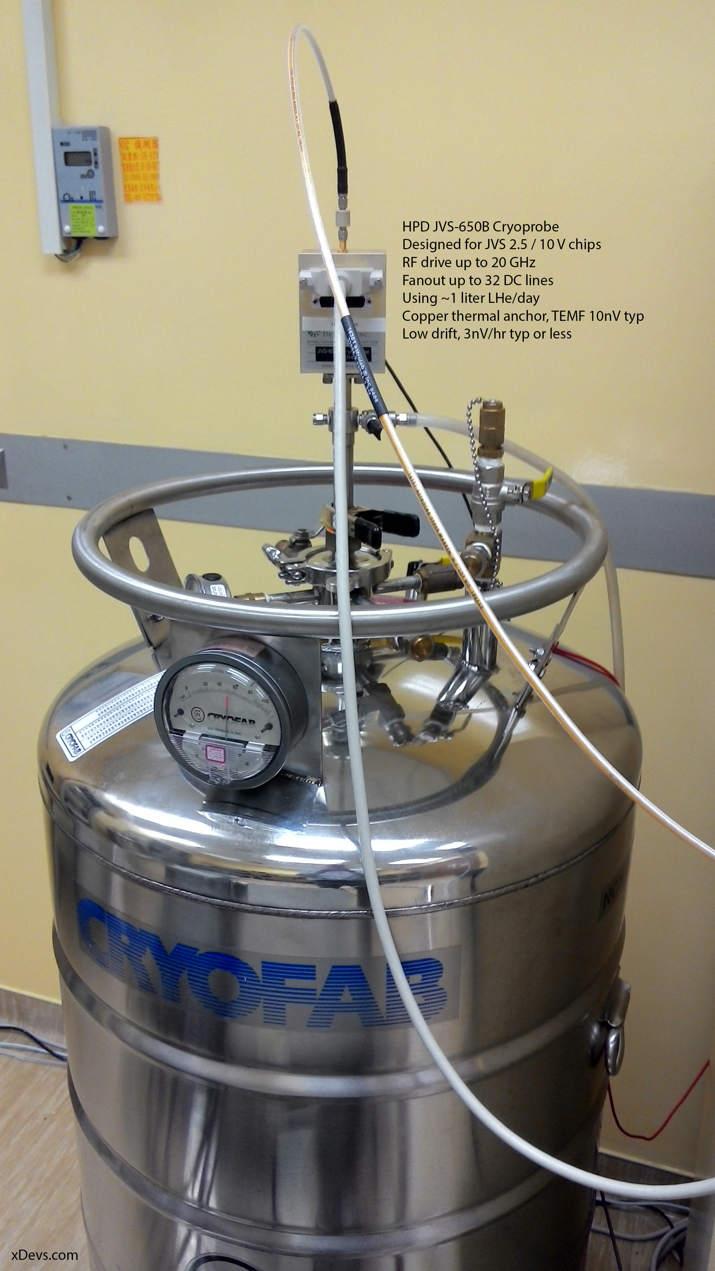
Image 41: Cryogenic hardware. Manometer shows helium level at about 50 liters
As the system operates, helium vapor vents through a gas valve for further recovery. This valve visible on the cryoprobe top flange with tube back to lab’s helium recycle system. Helium recycle is an important factor, because this light gas is a limited non-renewable resource on Earth and must be preserved. Earth atmosphere cannot prevent such light and inert helium gas from leaking into space.
Liquid helium cooling is one of few ways to reach ultra-cold temperatures and it is essential to high-energy physics experiments, use of superconducting materials, low-noise detectors operation and new material research. After the discovery of superconductivity effect, liquid helium allowed discovery and practical use of Josephson effect, the quantum Hall effect, superfluidity and modern research in quantum computing. One of the key fields relying on liquid helium coolant is NMR imaging in the fields of medicine, chemistry, pharmacology, and physics. NMR allowed research and synthesis of organic chemicals that have led to new drugs, plastics, and many related products.
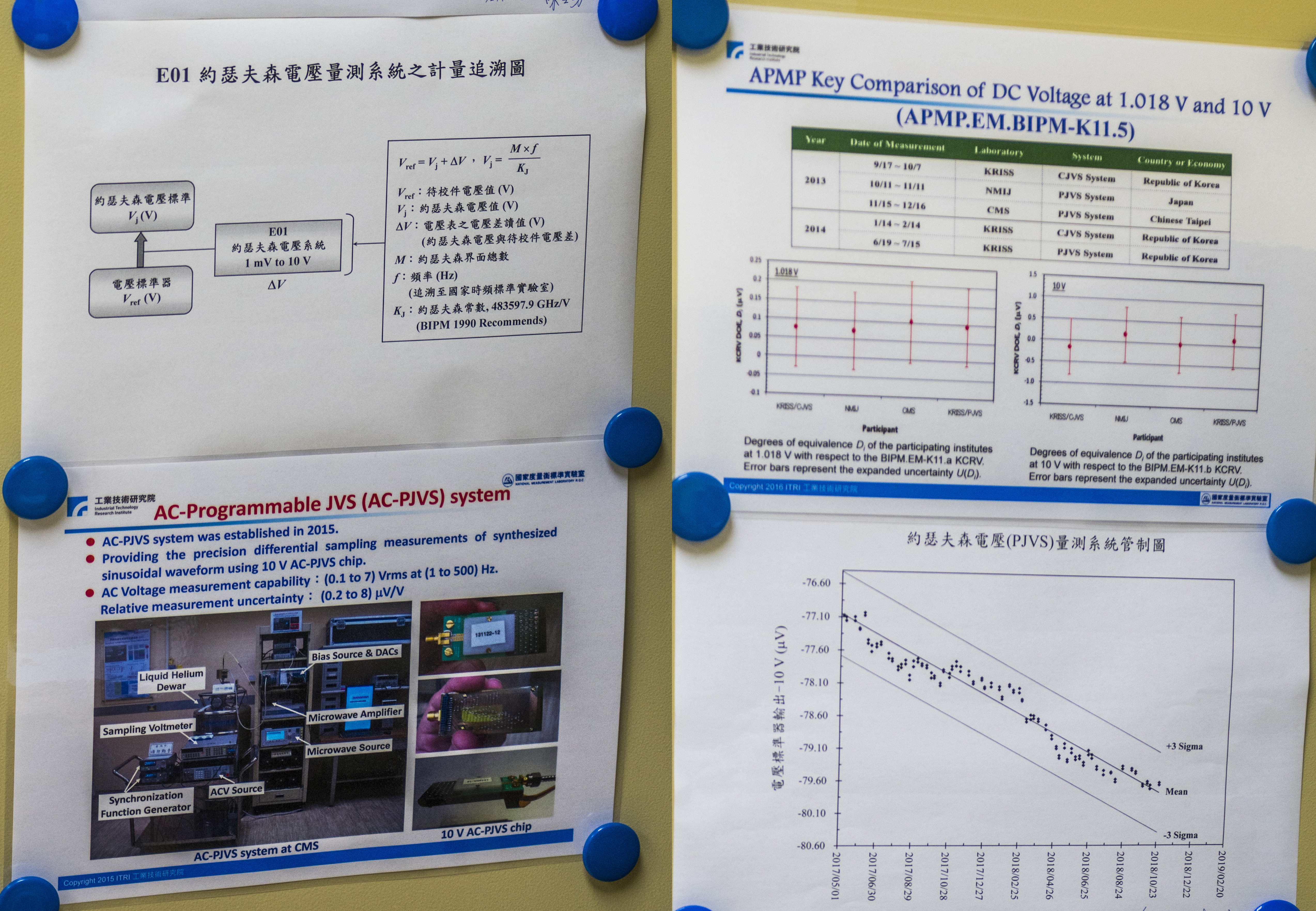
Image 42: PJVS chip traceability datasheet
CMS also have retired older CJVS system, that is based around an older 75 GHz voltage biased Josephson chip. Conventional JVS system requires special mmWave hardware to radiate Josephson Array with high-frequency RF. Rack with related equipment is depicted for comparison purposes.
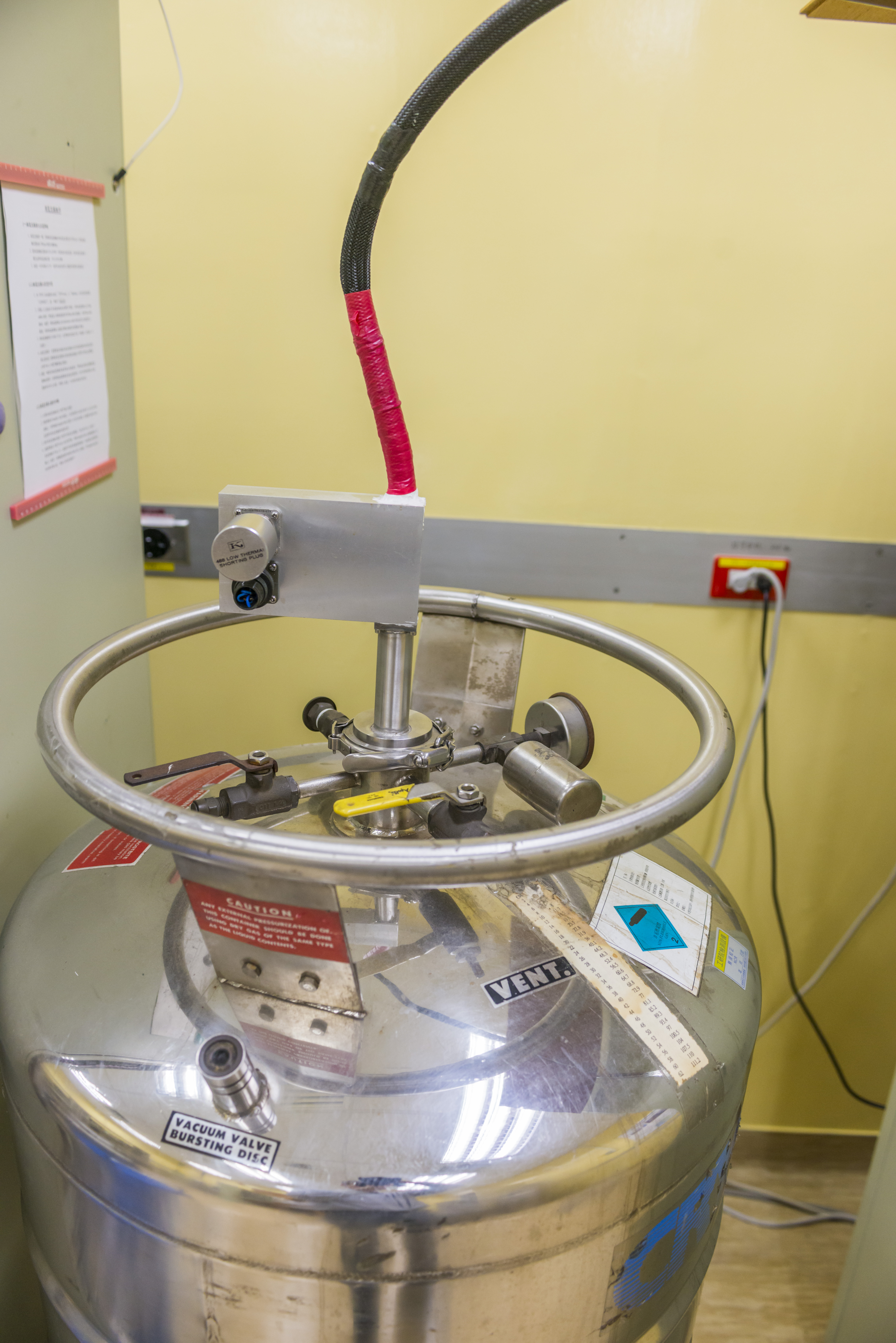
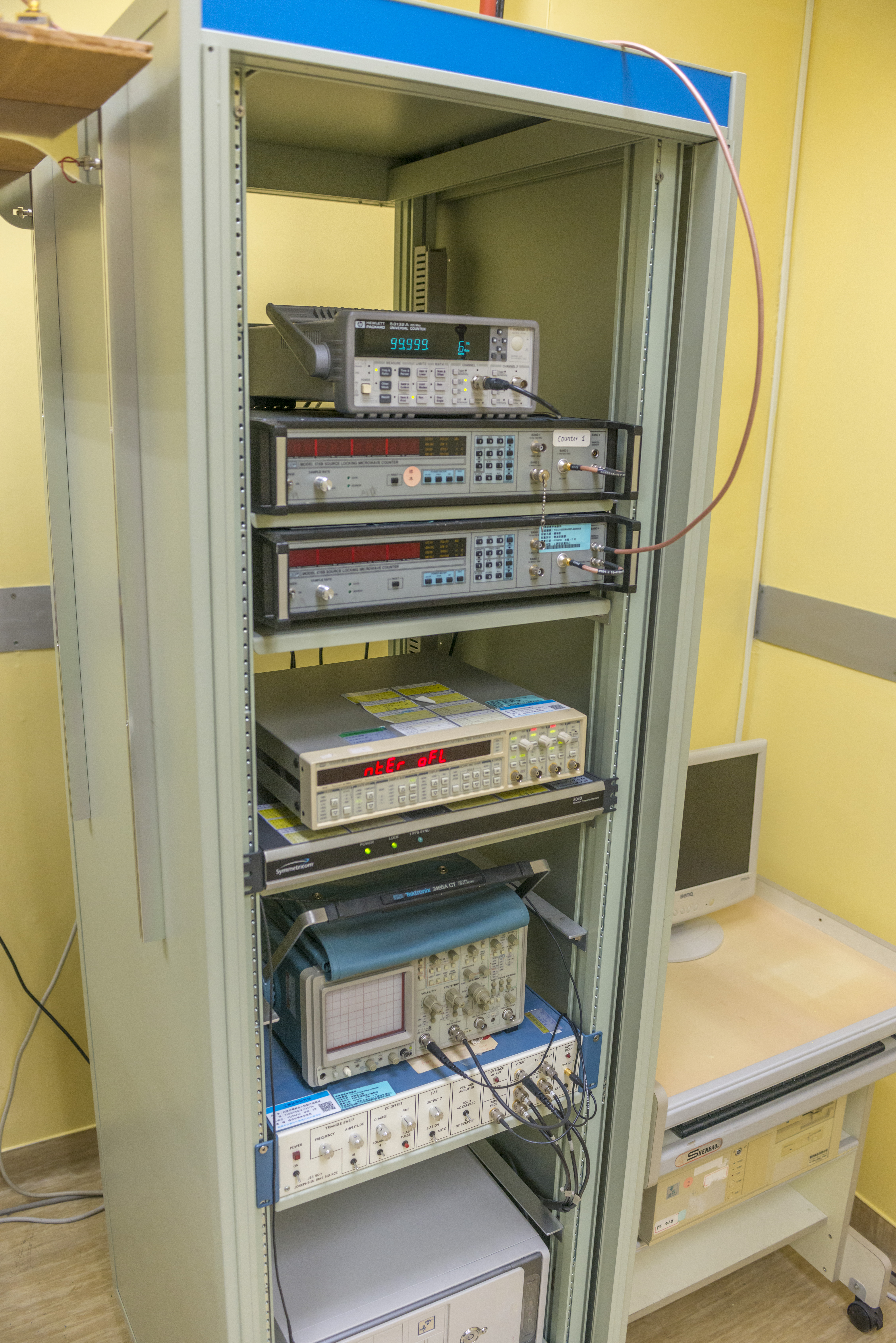
Image 43-44: CJVS system rack
To supply this mmWave field to JVS chip many CJVS use Gunn diode oscillator and locking counter, such as EIP 578. Counter measuring output 75 GHz signal from directional coupler with external waveguide mixer. Counter then generate correction signal to Gunn oscillator driver, that will adjust the output voltage to correct an error in 75 GHz RF output. Reference for the counter is also usually ultra-stable 10 MHz from Rb/Cs standard, just like in modern PJVS rig. This 75 GHz output is then filtered and routed to the CJVS chip in helium dewar via dielectric waveguide and cryoprobe interface.

Image 45: RF mixer, directional coupler, DC block, filter and waveguide interface
Mechanical RF attenuator is used to adjust signal strength for particular sweet spot stability of the CJVS chip/voltage point. Modern PJVS adjusts and maintains output power automatically with software control.
Resistance Laboratory
Resistance Standard lab is just across the hall, in close proximity.
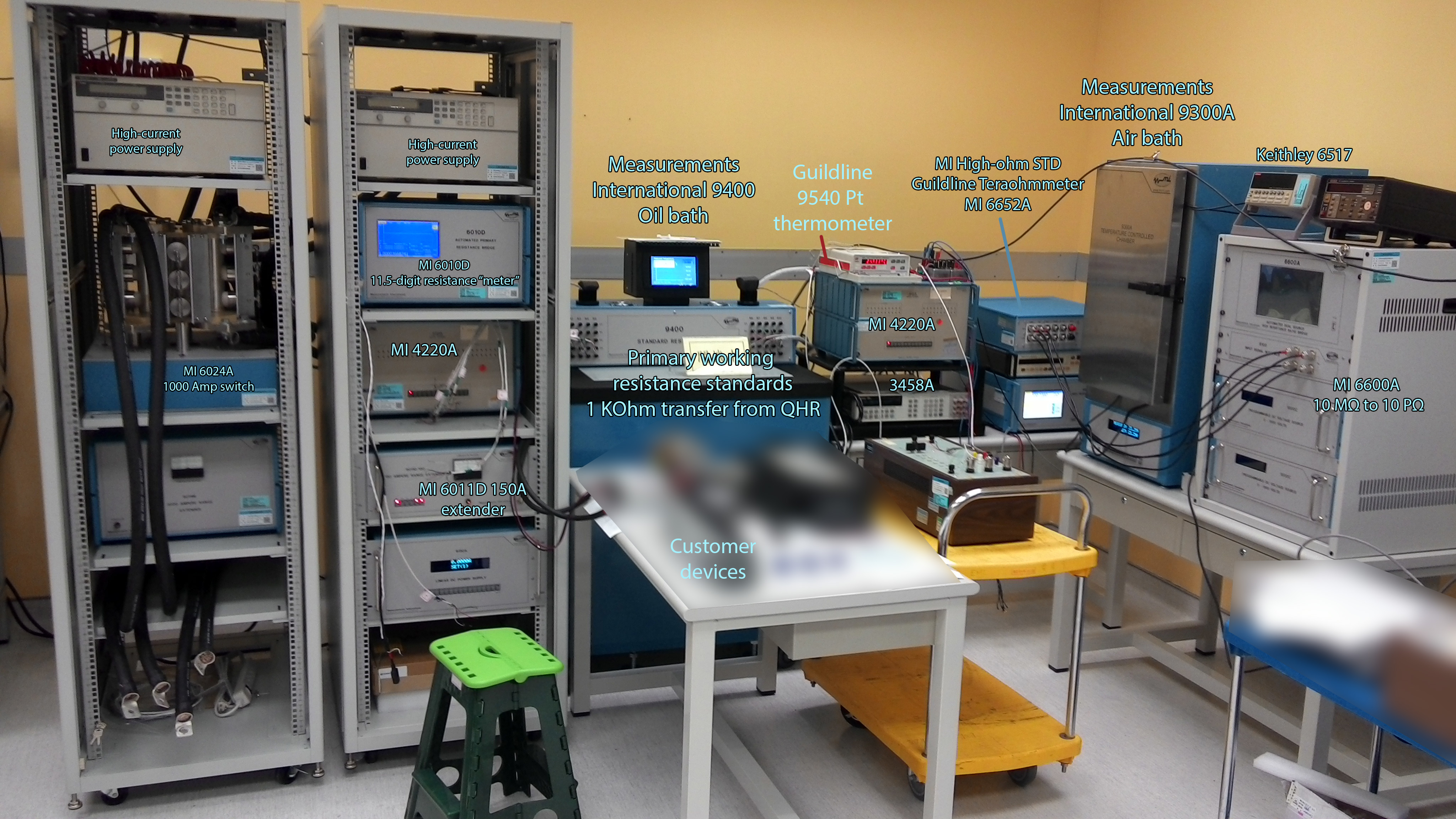
Image 46: Resistance lab equipment
This lab is literally filled with expensive Measurements International equipment and all kind of resistance gizmos.
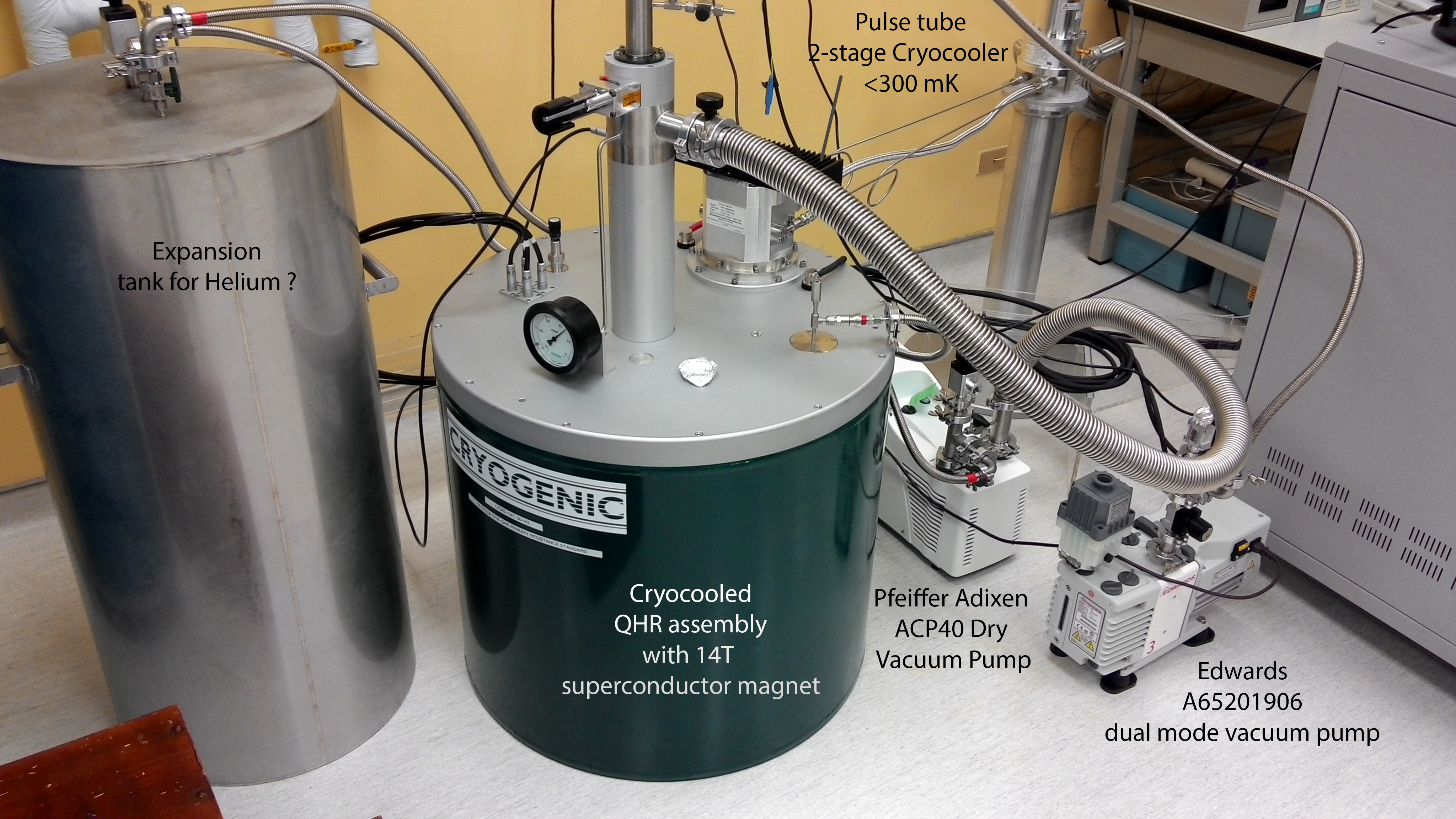
Image 47: Quantum Hall Effect Primary Resistance system with closed cycle
Primary resistance is realized by closed-loop helium-cooled apparatus and GaAs QHR chip from PTB. Just like JVS, Quantum Hall effects occurs only at very low temperatures below -270 °C and in strong magnetic fields. Corresponding vacuum-sealed cryogenic system and a superconducting solenoid are required for QHR operation.
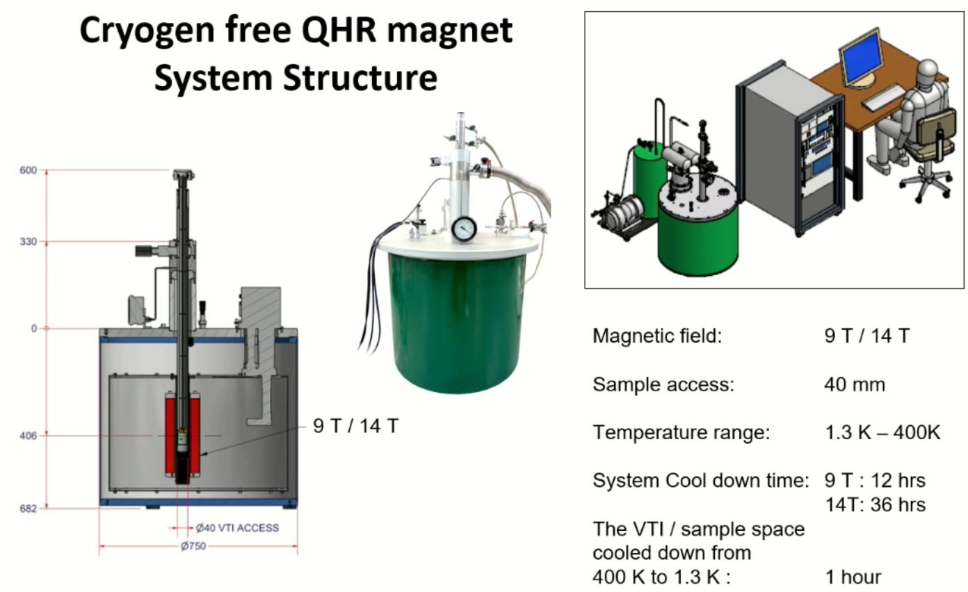
Image 47: Cryostat manufactured by Cryogenic Inc.
GaAs heterostructures became the established material at a temperature below 1.5 K and in a magnetic field of typically 10 T.
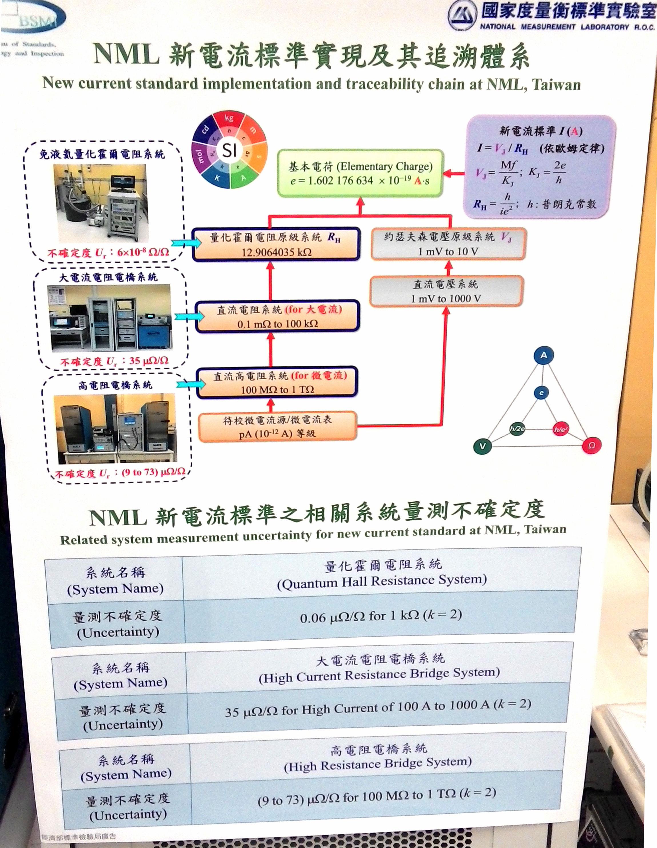
Image 48: Resistance lab transfers path
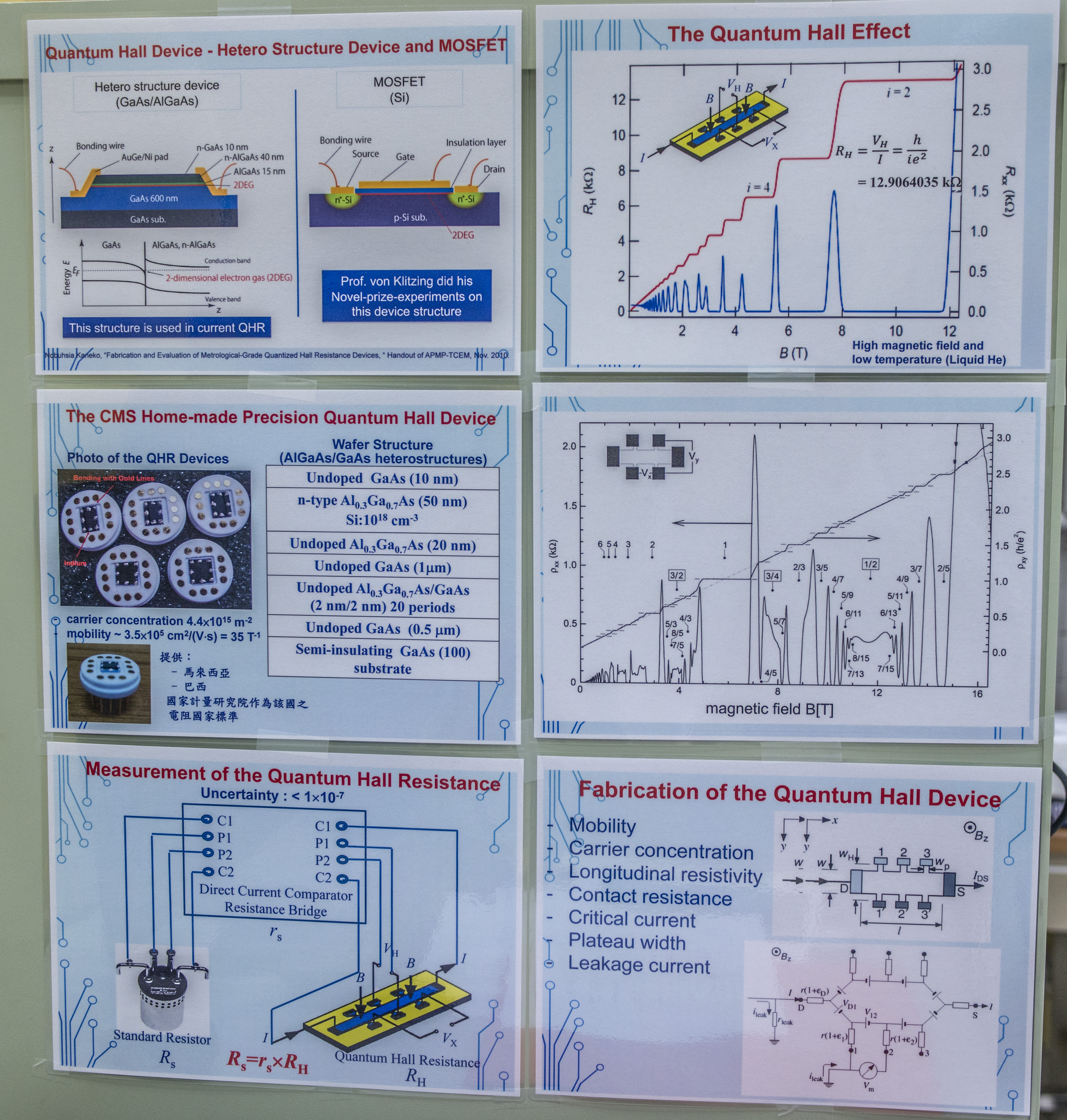
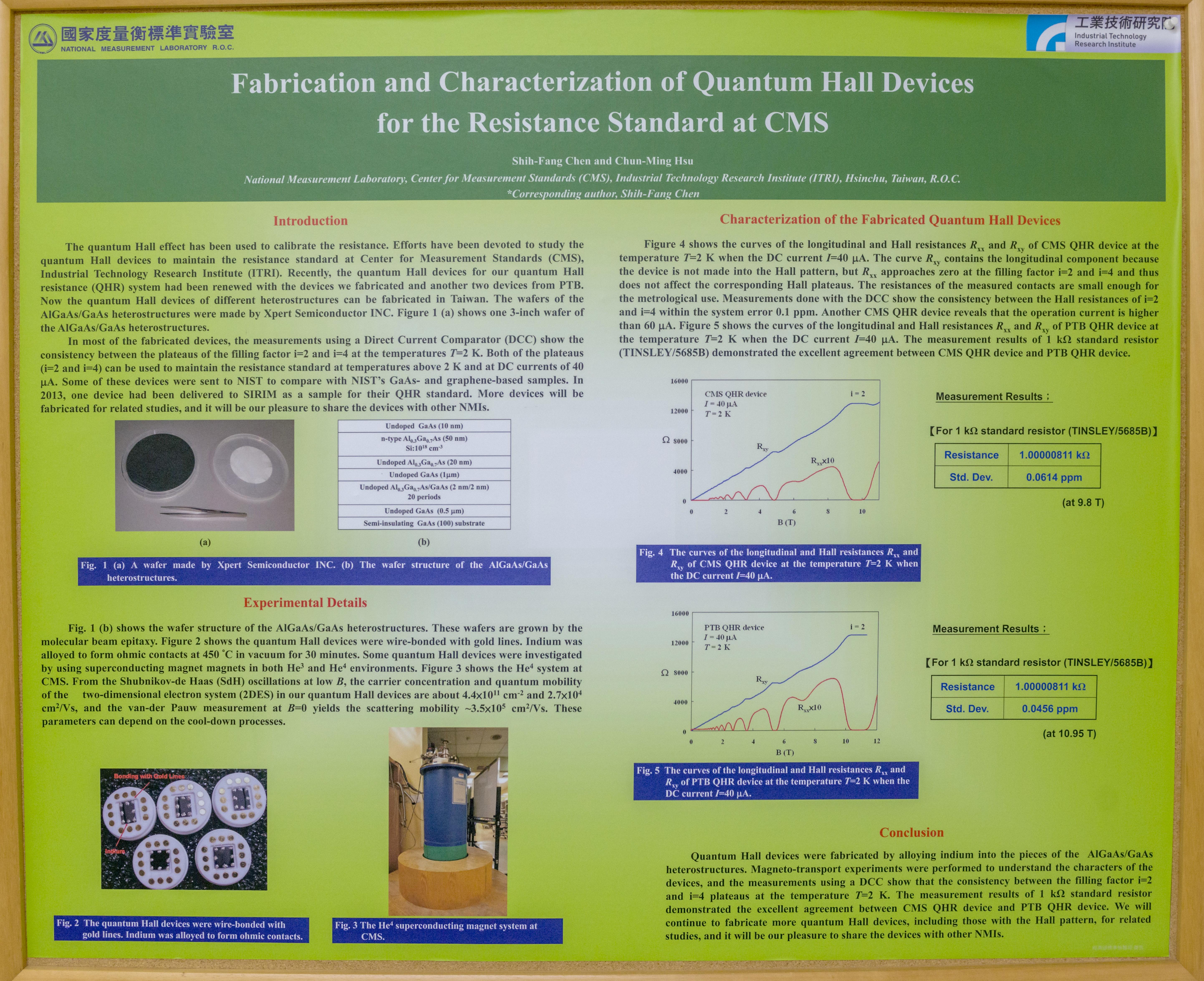
Image 49-50: CMS’s QHR chip design theory and PTB QHR device information
Intermediate stages in QHR chamber are cooled to ~54K and 4.7K. While this cooling system does not require refills for liquid helium tank, it consumes a lot of electrical power (~7 kW from 3-phase mains) to enable such low temperatures for 24/7 operation.
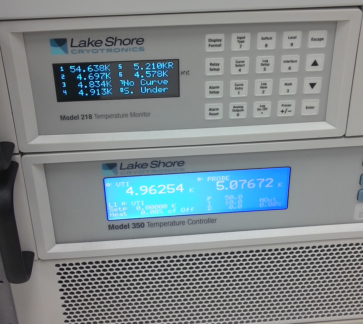
Image 51: Temperatures in the vacuum chamber while the QHR system in operation
| CMS calibration tier | E13 | E25 | E14 |
|---|---|---|---|
| Reference | Primary Resistances in Oil bath (verified by QHR) | Same as E13 | High Resistance Standard |
| Calibration DUT Resistance | 0.1 mΩ – 100 kΩ | 100 kΩ – 100 MΩ | 100 MΩ, 1 GΩ, 10 GΩ, 100 GΩ, 1 TΩ |
| Uncertainty | 0.1 – 4.2 µΩ/Ω | 6 µΩ/Ω – 16 µΩ/Ω | 0.09 mΩ/Ω to 0.6 mΩ/Ω |
| Estimated price | $345 USD per value | $345 USD per value | $145 per value |
Table 6: Resistance calibration services from ITRI CMS (June 2019)
SI Ohm Primary reference realized by cryocooled Quantum Hall Effect system. This system can provide and maintain quantum-accurate resistance 12906.4037296… Ω if used with i = 2 steps. Traceability obtained with QHR chip from PTB lab, but ITRI CMS also manufacture and test their own in-house designed QHR chips. Uncertainty of this resistance output is about 0.06 ppm, due to thermal and parasitic effects.
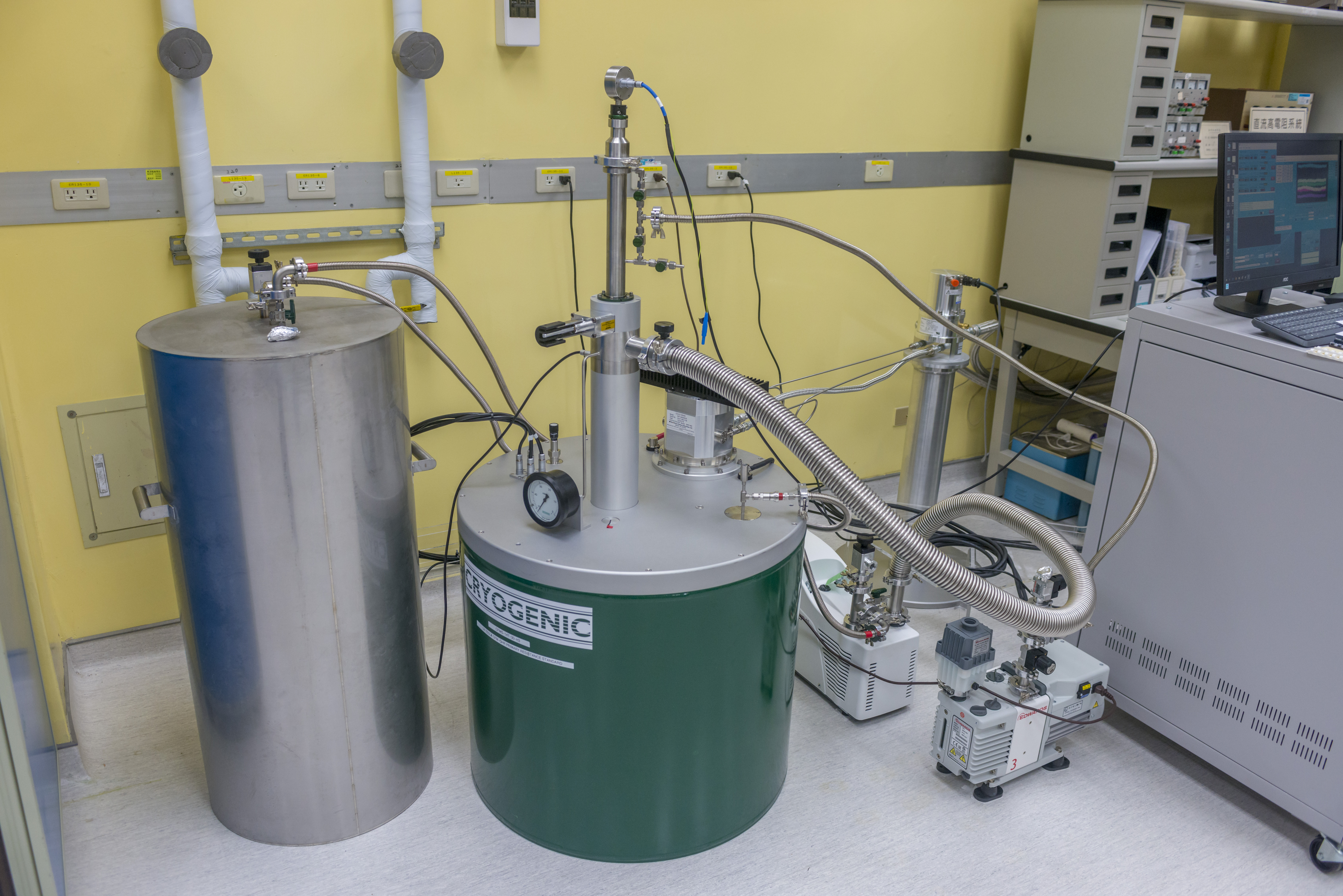
Image 53: QHR system, vacuum pumps and interconnects
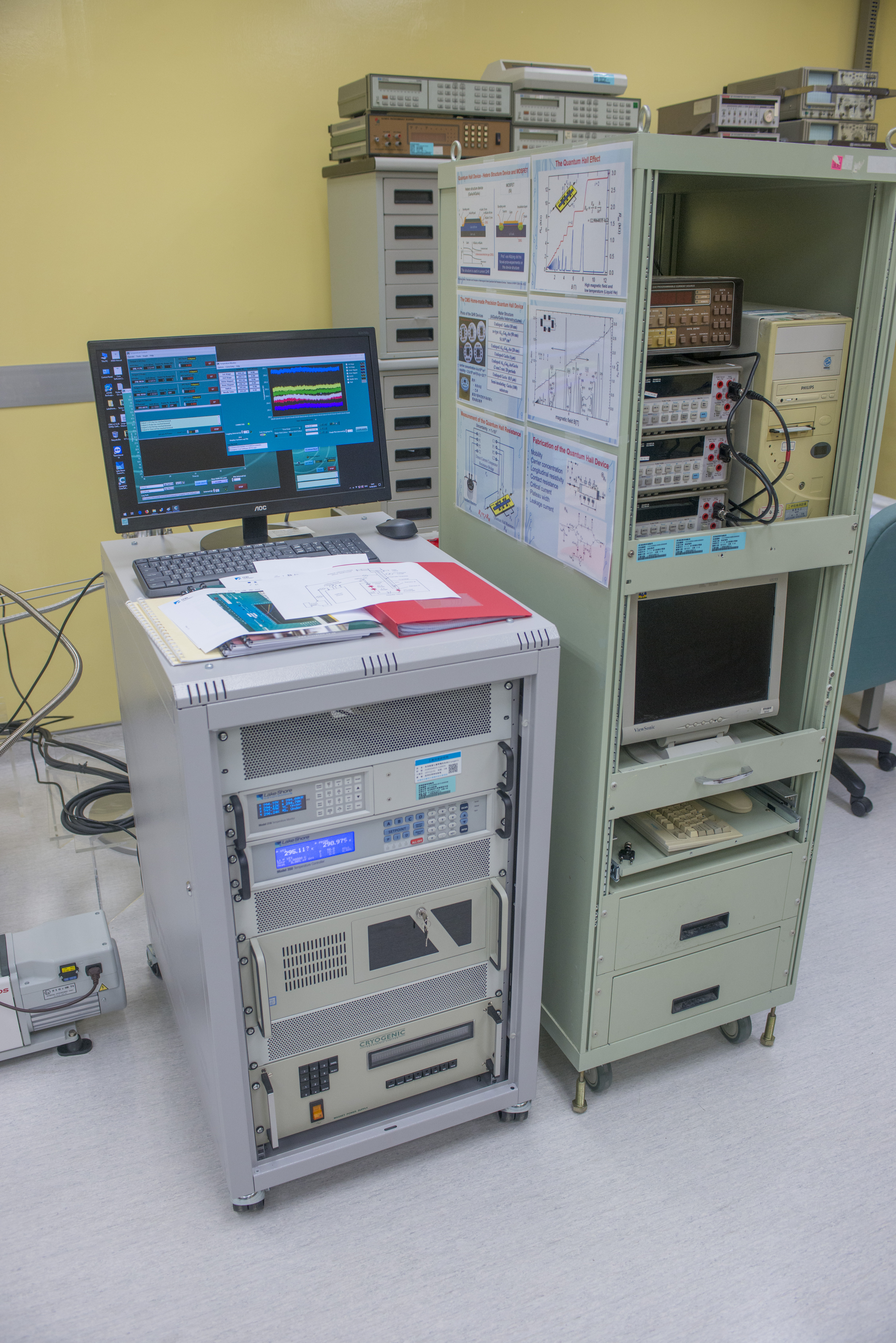

Image 54-56: Control rack for QHR with Lakeshore thermometers, magnet supply and PC
CMS also have older Liquid Helium cooled QHR setup, that sometimes used for testing experimental devices. It was not in operation during our visit to the laboratory.
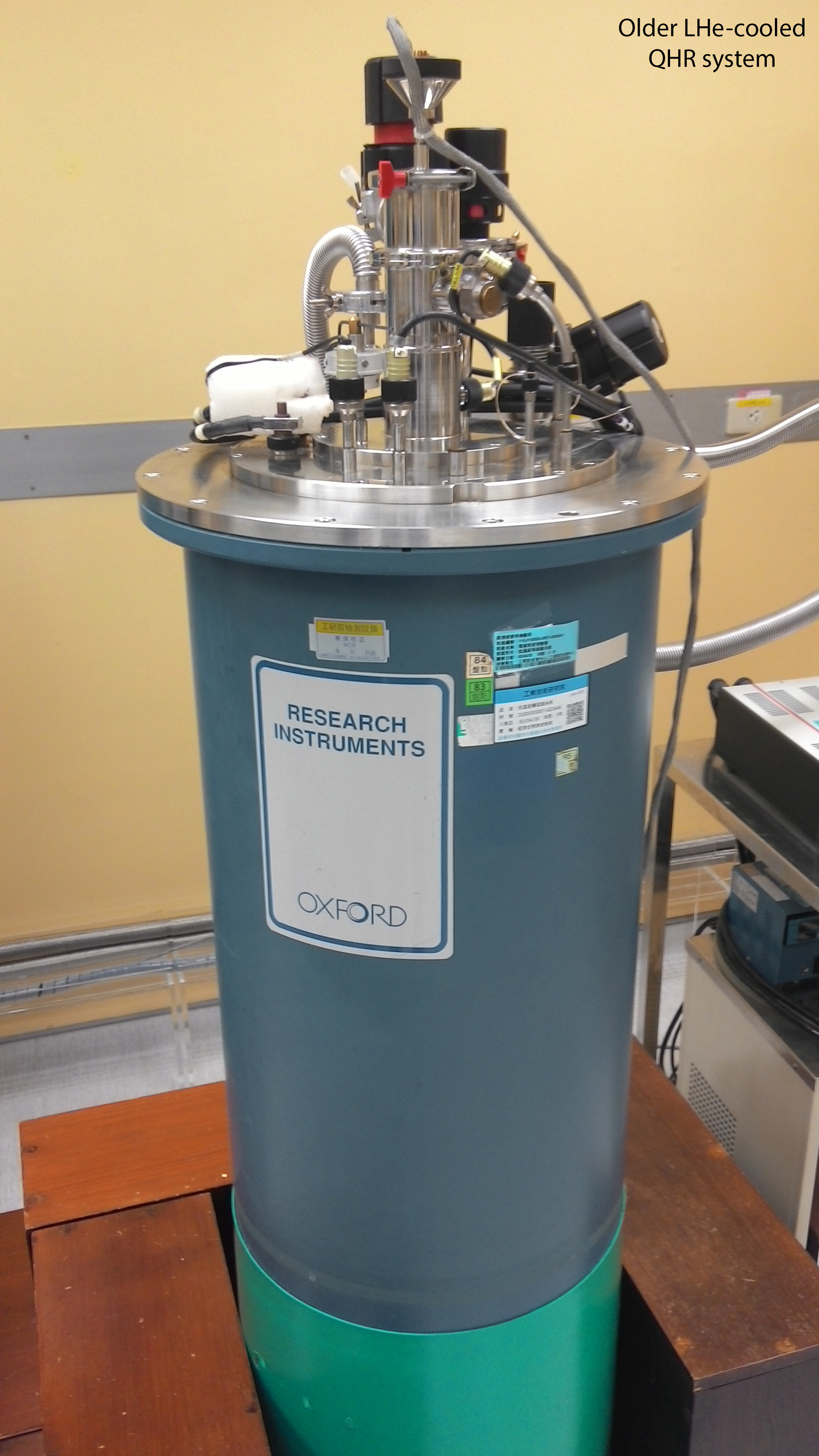
Image 58: Old QHR system using traditional liquid helium dewar

Image 57: Old system with related pumps and supporting apparatus
Unlike JVS setup, this Quantum Resistance cannot be programmed to arbitrary values, so external very high resolution ratiometric measurements are performed with help of DCC rack. First resistance is transferred to cardinal point ultra-stable wire-wound resistors, manufactured by Tinsley, MI, Guildline.
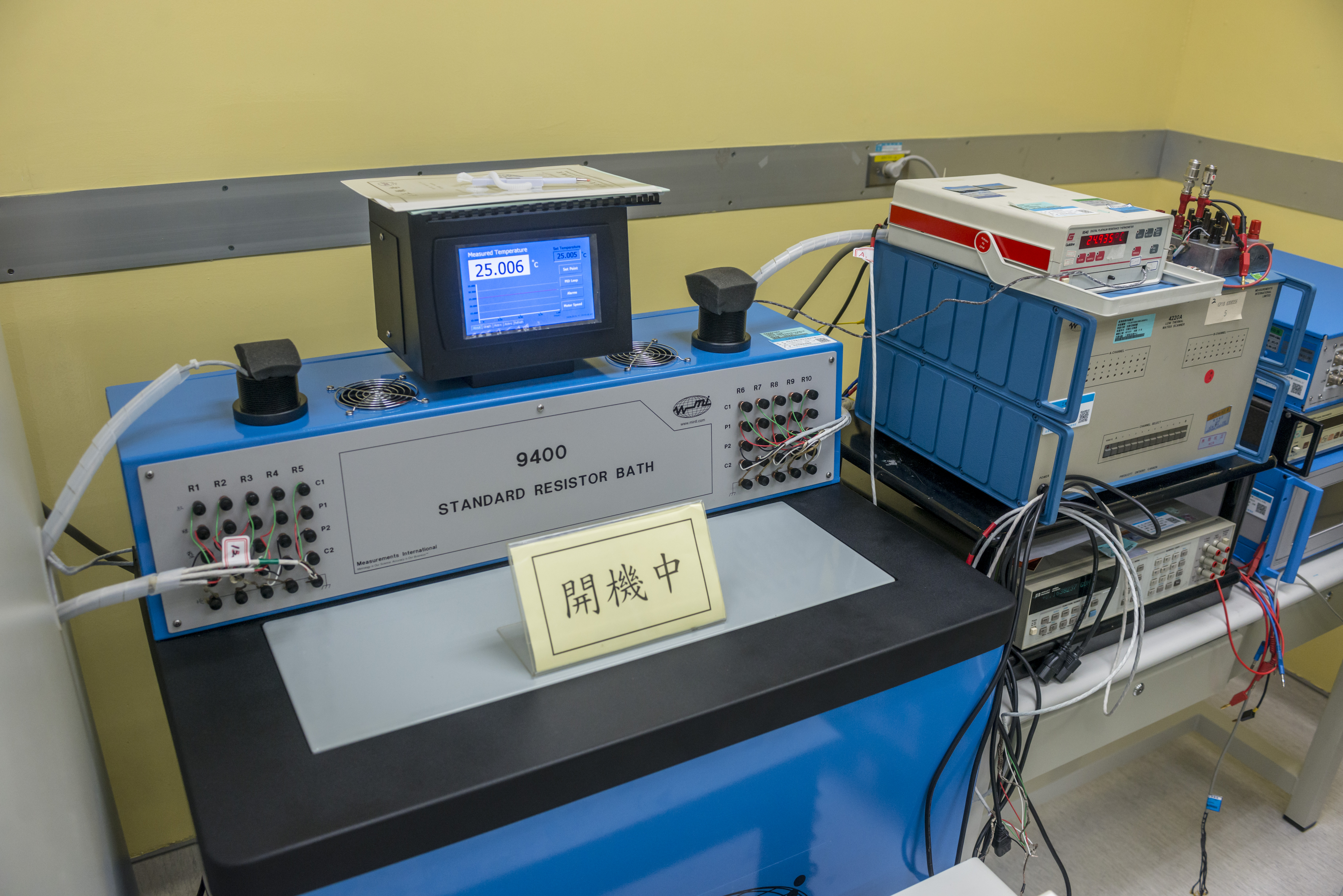
Image 60: National Resistance standards in MI 9400 oil bath, kept at constant +25.00 °C
Taiwanese National Ohm resistance set sits in Measurements International 9400 Oil bath thermally controlled tank. This bath maintains 75 liters of oil at constant +25°C temperature with stability <0.002 °C. The temperature in the bath can be programmed by the GPIB/RS232 interface. This unit can cool or heat oil in the bath using Peltier elements.
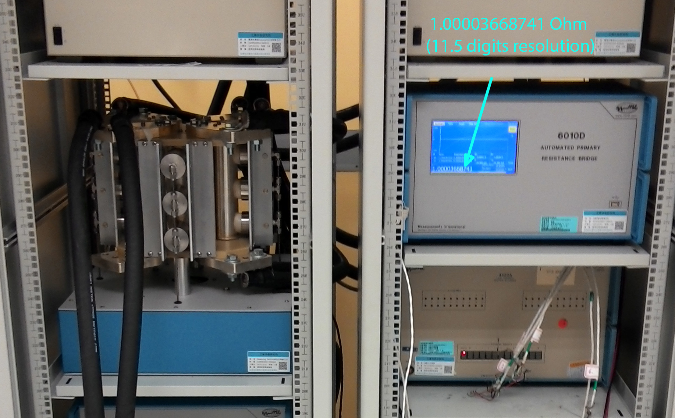
Image 61: 11½ digits resolution from MI 6010D. That is 10 picoohm on 1Ω range.
High current switch and current sources used to measure high-power shunts used in applications like industrial power meters, high-power experiments, battery, and power supply design and energy conversion industry.
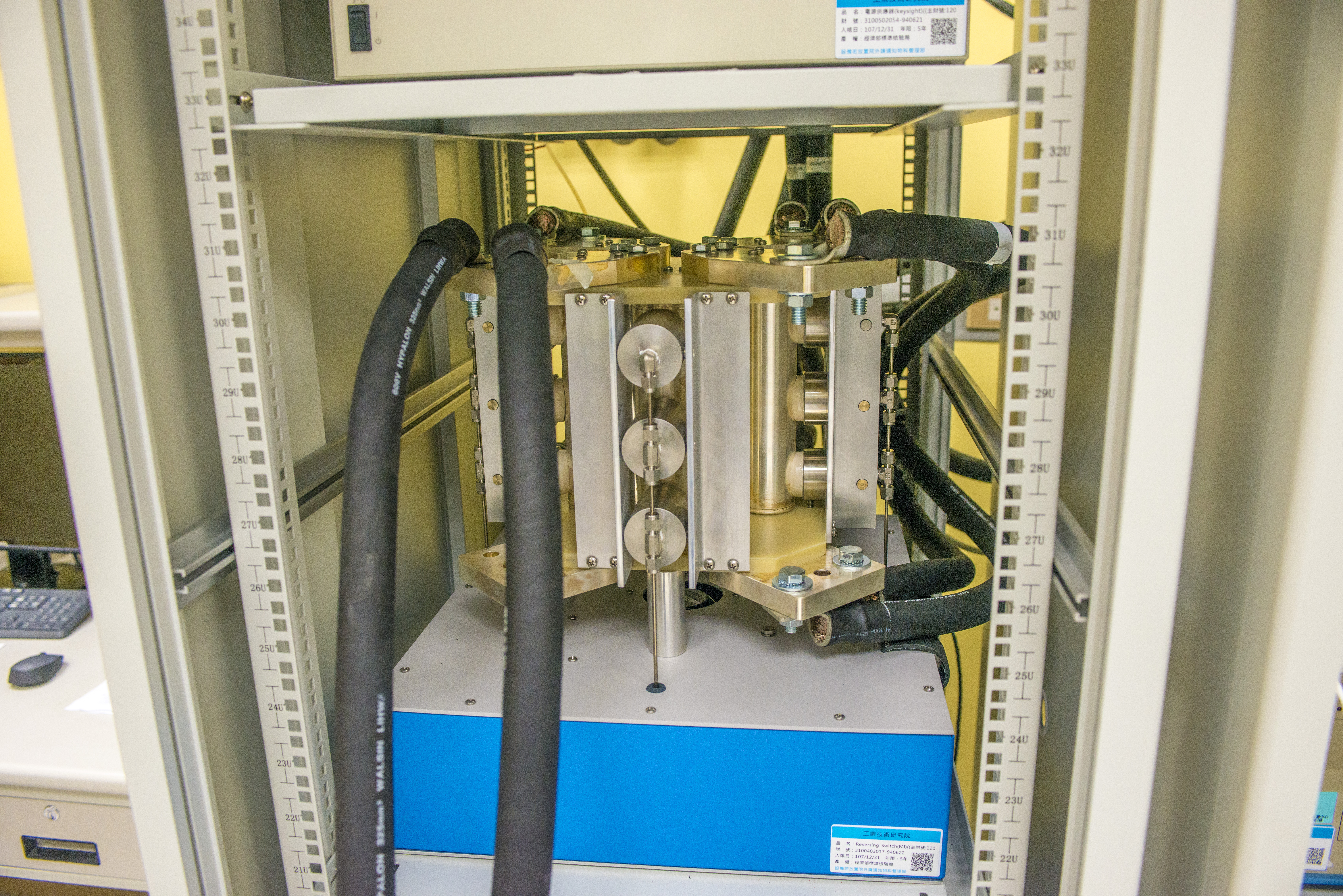
Image 62-63: MI 3000A reversal switch (left), Guildline oil bath
Image 64-65: MI DCCT racks with resistance bridge, extenders, current sources and 3000A switch
Typically high-accuracy resistance measurements use direct current comparator bridges, such as Measurements International 6010. Here we have latest version 6010D, able to perform ratiometric resistance transfers with resolution up to 11½ digits for resistances 0.001 Ω to 100 KΩ. Bridge have accuracy specification better than 0.04 ppm on 1:1 or 10:1 ratios, and linearity better than 0.005 ppm.
Bridge is configured in tall 42U 19-inch rack with 4220A Low thermal matrix scanner + MI 6011D (150 amp) + 6014M (3000 amp) current extenders. MI 4220A scanner allows automatic switching between different standard resistors to cover all resistance ranges in an automated manner, which is useful for multi-resistance standards calibration or MFC verification. Scanner has 20 4-wire low thermal inputs using tellurium copper contacts and terminals with two 4-wire outputs. All switching relays are hermetically sealed and support 250 Volts or 4A of current. Thermal EMF error contributed by the switch is specified less than 20 nV, while insulation resistance is in excess 1014 Ω.
High DC current sourced by not one, but two Keysight 6680A 5000 Watt power supplies. Each of these beasts can source up to 875 Amp. Interesting enough, Keysight discontinued these PSUs, with no alternative offering for such high currents on site?
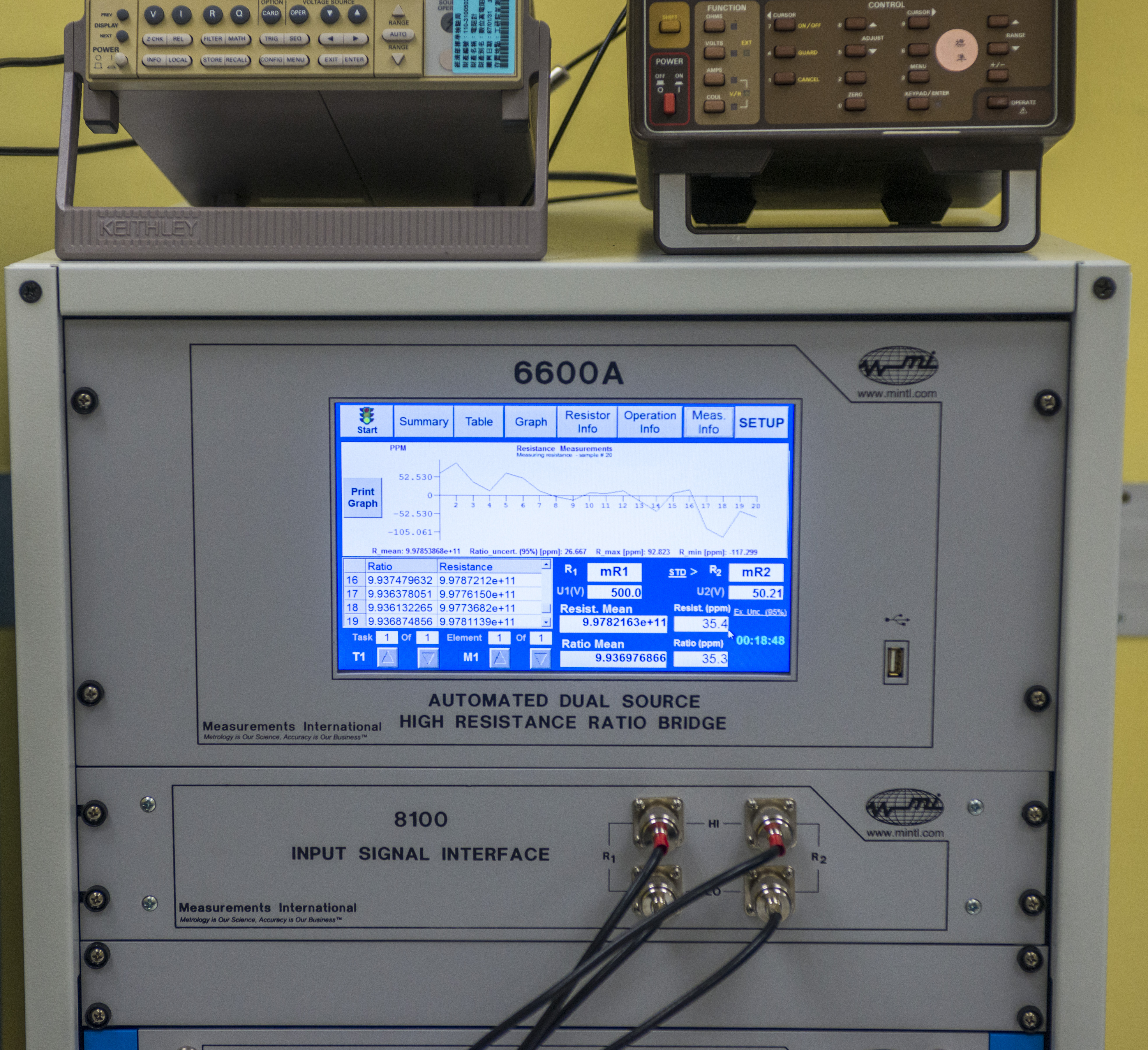
Image 66-67: MI 6600A system and MI air-bath for resistance tests
Higher than 100 kΩ resistance is handled by yet another station, around Measurements International 6600A rack. This setup can perform bridge or direct fully guarded measurements for resistance from 100 kΩ to 10 PΩ (1015 Ω!). There are two MI 1000C low-noise precision voltage sources in the system, both supporting voltage up to 1kV.
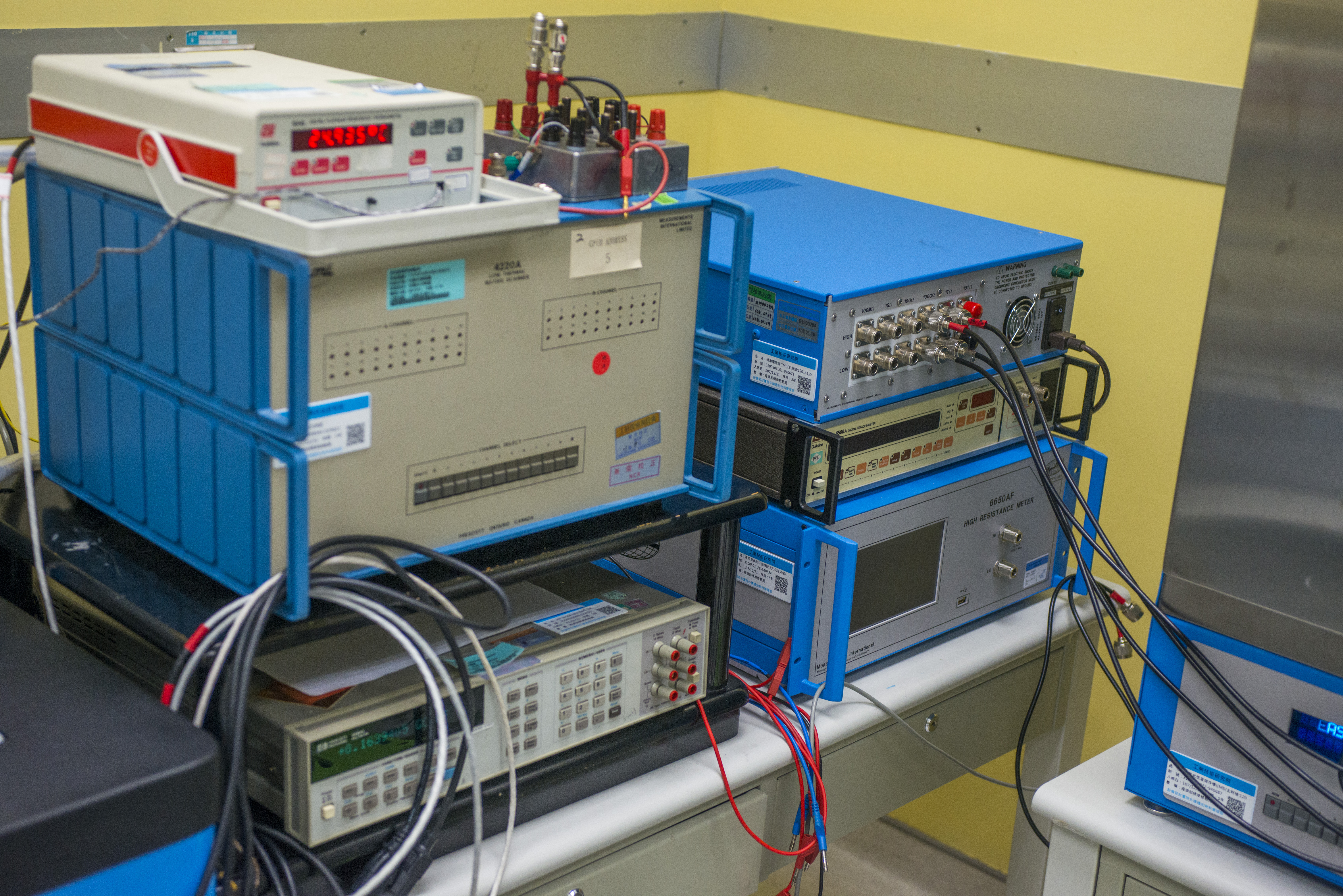
Image 68: Measurements International 6500AF system, Guildline 6500 and MI scanner
Smaller MI 6650AF system also can cover resistance ranges from 100 kΩ to 100 TΩ but provide less accuracy and resolution.
Use of multiple different bridges is important to obtain the best possible uncertainty for specific points. There is no one magical instrument that can provide the best result on every possible calibration job. Graph from MI illustrates that well, showing the capability of different type bridges.
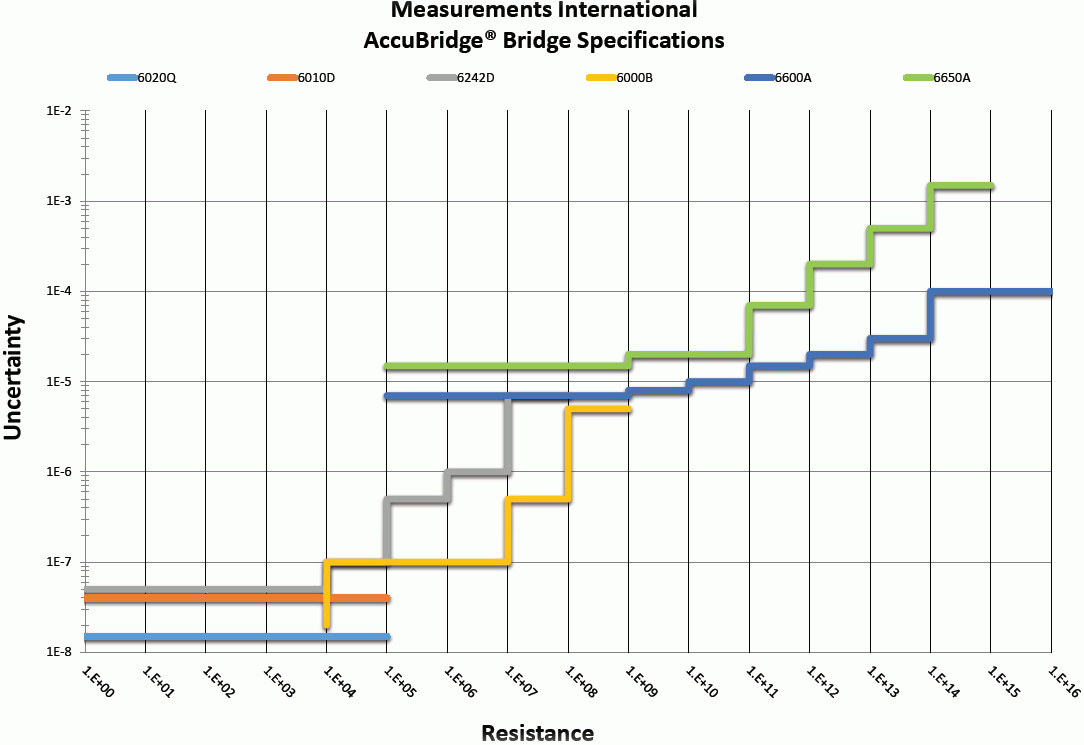
Image 69: Transfer uncertainty of Measurements International bridges. Courtesy MI marketing.
AC Voltage/Current Laboratory
To maintain low-frequency precision AC voltage and current calibrations CMS using a set of characterized thermal converters, coaxial Fluke A40B shunts, Fluke 792A AC/DC transfer standard, and calibrators.
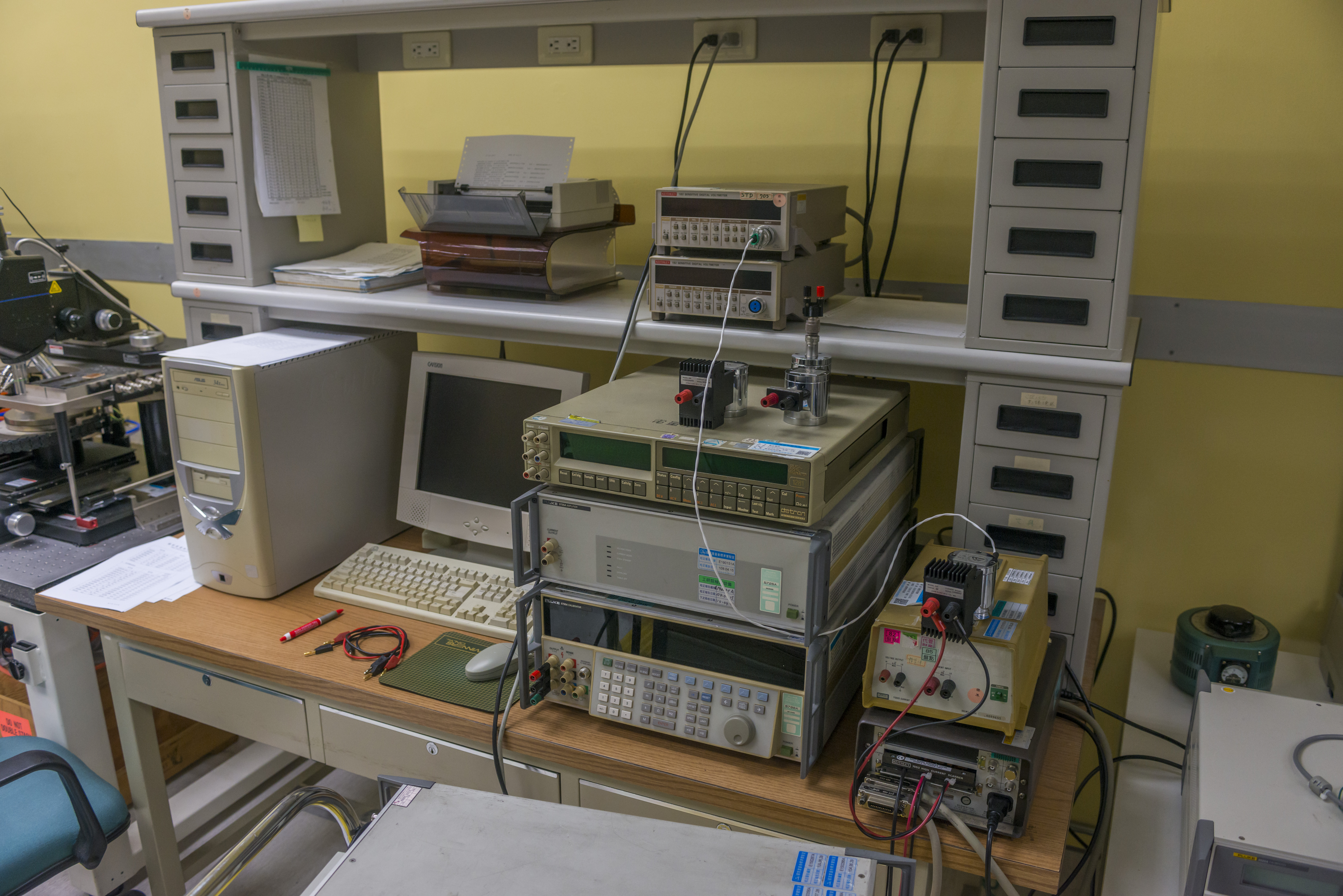

Image 70-71: Fluke 5700+5725 and Datron 1281 (left), Fluke 5730A, 5790B, 52120A (right)
In AC lab we can see Fluke 5790B AC/DC transfer standard recently released in 2016, Fluke 5730A high-end multi-function calibrator, together with Fluke 52120A high-current trans-impedance amplifier.


Image 72-73: Thermal converters and AC shunt inventory at CMS AC Lab
Calibration results
ITRI CMS Lab is approved and certified by BIPM via participation in key comparisons. This is public information, published on BIPM site
BIPM Record from KCDB, ITRI CMS expanded uncertainties for electricity, November 2016
Round 1 – May 2019
On arrival to the CMS, both standards were inspected to confirm safe transport, and Fluke 732B was plugged to mains power to maintain battery charge. A few hours later short test was performed, taking a measurement on automated solid-state zener bank measurement system, to confirm good and stable 10V DC output from our 732B. The unit left to settle after transport stress for 4 days, and calibration versus Josephson Voltage System has performed afterward on May 31, 2019. DC Standard was operated on battery power during the measurement.
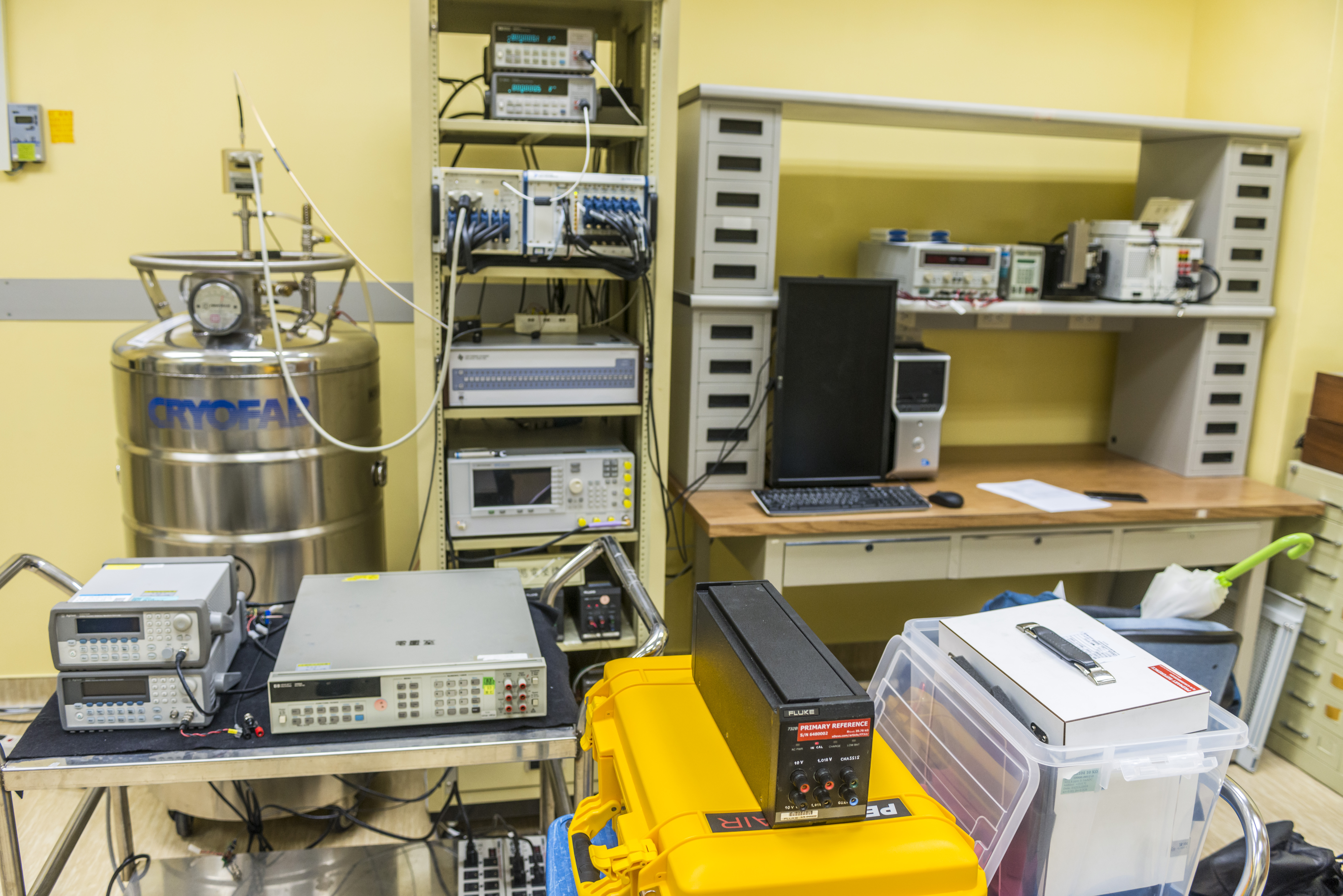
Image 59: xDevs.com’s 732B and ESI SR104 transfer units in DC Standards Lab
NMI Calibration report for Fluke 732B DC Voltage Standard
Calibration report expanded uncertainty for our DC standard is tiny 0.02 µV/V, which translates into 0.02 ppm at 10 VDC output level. This is so small, that standard essentially will drift outside of this uncertainty just in term of a few days. If we take Fluke’s specification for 90 days, maximum drift is listed at ± 0.8 ppm. Uncertainty valid period estimation on this worst-case scenario can be roughly done by box method:
Drift 0.8 ppm / 90 days = 0.008888… ppm per day. UCAL_JVS0.02 ppm / 0.0008888… = 2.25 days
Even if particular 732B is 10 times better than its specification, that would still make own 732B surpass uncertainty of the direct calibration against JVS in less than a month.
So paying extra for JVS calibration on solid-state standards is a waste of money? Well, not so simple. If we perform multiple calibrations over the longer time span, all with this level of uncertainty, for example, every month during a year, it would be possible to build actual DC output prediction statistics model, and future calibrations would be done to maintain that VPREDICTED with good uncertainty. All solid-state references drift, but that drift usually stays constant in magnitude when the standard is undisturbed by external influence and power. This way we can “override” specifications provided by Fluke and use our own data to obtain sub-ppm accuracy over longer time span. In fact, Fluke even has a public white paper touching on this subject.
NMI Calibration report for ESI SR104 Resistance Standard
ESI SR104 used for transfer allowed to soak at constant +23.000 °C air bath (Measurements International) for 4 days before actual measurement with DCC bridge (Measurements International 6010D) occur. Current used by the 6010D during measurement was set to 100 µA for 10 kΩ standard resistor in order to limit power coefficient and thermal heating effects. Because ESI SR104 is hermetically sealed resistor element in the oil bath, humidity is not considered as significant error factor.
Deviation of this particular SR104 is 0.0 ppm, according to lid note from June 2003 calibration, while actual certificate report from May 2016 reported 10000.0011 Ω measurement result, but the uncertainty of that reading is ± 1.0 ppm due to use Fluke 8508A-001 and other ESI SR104 as standard.
This calibration by ITRI CMS assigned resistance value 9999.9995 Ω with combined uncertainty just ±0.16 ppm. ESI SR104 standard was kept at constant temperature +23.000 °C in Measurement International 9400 air bath for multiple days before and during measurements.
Actual measurements were taken in a period of 4 days from June 3, 2019, till June 6, 2019, with MI 6010D DCC bridge system and primary national resistance standard with nominal 1000 Ω.
Because calibration took place during own CMS lab calibration cycle for all their primary resistors, QHR system was used to calibrate 1000 Ω standard at the same time, June 3, 2019. Even calibration report for our ESI SR104 is just 1 digit later to CMS’s own 1000 Ω. This means that error of DCC transfers between intrinsic primary standard like QHR system to 1000 Ω in the oil tank and followed by calibration our ESI SR104 10000 Ω is minimal, and most likely well below even 24-hour specifications of the MI 6010D system. As a result our SR104 received “golden” calibration, in some meaning, with uncertainty way below what is possible at even fully stuffed commercial calibration house.
Fellow metrology enthusiast Lymex had significant effort to collect data on many ESI SR104’s to estimate typical drift rate of these amazing resistance standards.
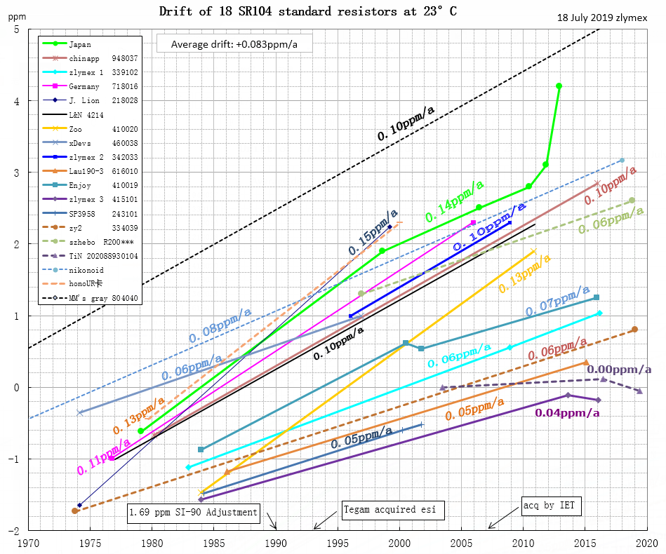
Image 74: Drift rates of 19 different ESI SR104 resistance standards, per year
Based on his research, worst SR104 out of 17 units have drift just +0.15 ppm per year, which is far below any commercial resistance standard specification available. This again confirms the exceptional performance of these old ESI SR104 standards.
Round 2 – August 2019
NML Calibration report for xDevs.com’s Fluke SL935 Heated Resistance Standard
Our special Fluke SL935 resistance standard was traceably calibrated twice before, by Process Instruments in USA. Summary with results is shown below:
| Date | 10 KΩ | 1 Ω | 10K,ppm Δ | 1Ω,ppm Δ | Instrument | 10 KΩ Δ/day 0, ppm | 1 Ω Δ/day 0, ppm | Ambient, °C |
|---|---|---|---|---|---|---|---|---|
| 28 Nov 2017 0.3mA PI | 9999.9747 ±0.33 ppm | Reference | MI 6010B + L&N 4210 | Reference | +23.00 ±0.05 | |||
| 31 May 2018 0.3mA PI | 9999.9755 ±0.33 ppm | +0.08 ppm | MI 6010B + L&N 4210 | +0.000437 ppm/day | +23.00 ±0.05 | |||
| 10 Jan 2019 predicted | 9999.9764 | +0.17 ppm | Prediction | +0.000437 ppm/day | +23.00 ±0.05 | |||
| 4 August 2019, 0.1 mA | 9999.9774 | +0.27 ppm | Prediction | same | +23 | |||
| 13 August 2019 ITRI CMS NML 0.1 mA | 9999.9739 | -0.08 ppm | MI 6010D, TW Oilbath STDR | Same | +23.00 ±1.5 | |||
| 13 August 2019 ITRI CMS NML 0.3 mA | 9999.9737 ±0.17 ppm | -0.10 ppm | MI 6010D, TW Oilbath STDR | Same | +23.00 ±1.5 | |||
| 28 Nov 2017 100mA PI | 1.00005902 ±0.17 ppm | Reference | MI 6010B + L&N 4210 | Reference | +23.00 ±0.05 | |||
| 31 May 2018 100mA PI | 1.00005942 ±0.17 ppm | +0.4 ppm | MI 6010B + L&N 4210 | +0.00218 ppm/day | +23.00 ±0.05 | |||
| 10 Jan 2019 predicted | 1.00005991 | +0.89 ppm | Prediction | Same | +23.00 ±0.05 | |||
| 4 August 2019 predicted | 1.00006036 | +1.34 ppm | Prediction | Same | +23.00 ±0.05 | |||
| 13 August 2019 ITRI CMS NML | 1.00006085 ±0.17 ppm | +1.83 ppm | MI 6010D, TW Oilbath STDR | Same | +23.00 ±1.5 |
Calibration data summary and predictions
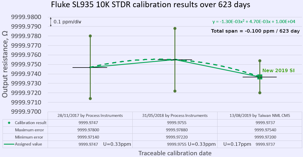
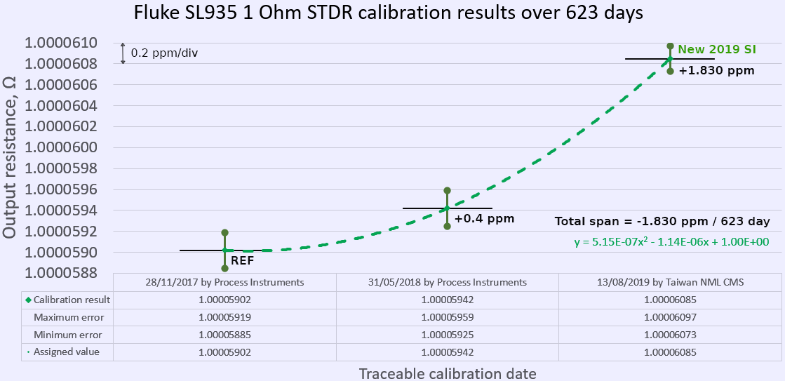
Here we can clearly see, that using small number of points with large time period between calibrations, even with very low uncertainty per each point does not provide enough information for accurate output predictions. This is why many metrology labs maintain and keep even obsolete and old equipment, as they have decades of calibrations and characterization attached to device. With brand new instrument, even at better specifications it will take many years to build up confidence good enough for sub-ppm predictions.
NML Calibration report for xDevs.com’s 792X DC Voltage Standard ‘FX’ LTZ1000A 10V output
After standards received their calibration, I have hand-carried them back to xDevs TW lab and final question was “And now what?”. Next two chapters answer that in a moment.
Transfer of voltage, using calibrated +10.000 V DC standard
Now after DC voltage output from transfer Fluke 732B calibrated with ±0.02 ppm uncertainty (10.0000152 V ±0.0000002 V) accurate transfers of the reference can be made into lab standards, long-scale DMMs and Fluke 5720A calibrators. This task must be performed as soon as possible, to minimize the error of own 732B drift. The table below summarize overall stability between our available DC voltage sources and meters.
| Device | 24 hour specification | 90 day specification | 1 year specification |
|---|---|---|---|
| Fluke 732B or 732C | < ±0.3 ppm (10V output), 30 day | ± 0.8 ppm | ± 2.0 ppm |
| Datron 4910 (1 cell) | < ±0.3 ppm (10V output), 30 day | ± 1.0 ppm | ± 1.5 ppm |
| Wavetek 7000 | < ±0.5 ppm (10V output), 30 day | ± 0.8 ppm | ± 1.2 ppm |
| Fluke 732A | < ±0.5 ppm (10V output), 30 day | ± 1.0 ppm | ± 3.0 ppm |
| xDevs.com 792X | < ±0.5 ppm (10V output) | ± 1.0 ppm | ± 3.0 ppm |
| Fluke 5720A | ±0.55 ppm (10V output) | ± 1.8 ppm | ± 2.8 ppm |
| HP 3458A/X02 | ±0.55 ppm (12V range) | ± 2.15 ppm | ± 3.05 ppm |
| HP 3458A/002 | ±0.55 ppm (12V range) | ± 2.66 ppm | ± 4.06 ppm |
| Fluke 8588A | ±0.6 ppm (20.2V range) | ± 1.5 ppm | ± 2.8 ppm |
| Datron 1281 | ±0.7 ppm (20V range) | ± 3.2 ppm | ± 3.2 ppm (w/Self-Cal) |
| Datron 4808 | ±0.8 ppm (10V output) | ± 4.0 ppm | ± 7.5 ppm |
| Fluke 8508A | ±0.9 ppm (19V range) | ± 1.8 ppm | ± 3.0 ppm |
| Keithley 2002 | ±1.4 ppm (21V range) | ± 6.3 ppm | ± 10.3 ppm |
| Keithley DMM7510 | ±2.84 ppm (12V range) | ± 10.44 ppm | ± 15.44 ppm |
Table 7: Standards/DMM/MFC DCV stability over different calibration periods
Based on specifications in table, sub-ppm accuracy for 10V DC output/ranges possible with use of Fluke 732B as standard only for a period less than 3 months. DMMs within the calibration period, even very expensive ones like Fluke 8508A can offer sub-ppm uncertainty when calibrated by 732B only for a period less than 24 hours, granted only if 732B standard itself have suitable calibration.
Top-level laboratory always has bank of multiple solid-state zener references such as Fluke 734A/C, Datron 4910 or Fluke 7004/7010N systems to improve confidence in such demanding accuracy levels without expense and complexity of Josephson Voltage System. Use of multiple references and a careful chain of calibration can help to obtain drift characteristics, which allow to “predict” output voltage at any given time, with decent confidence in sub-ppm uncertainty over a longer time span.
Back in 2016, our first transfer was completed using HP’s 3458A A9 LTZ1000A reference module, cross-shipped internationally between USA and Taiwan. Details of that simple travel “standard” explained in this article.
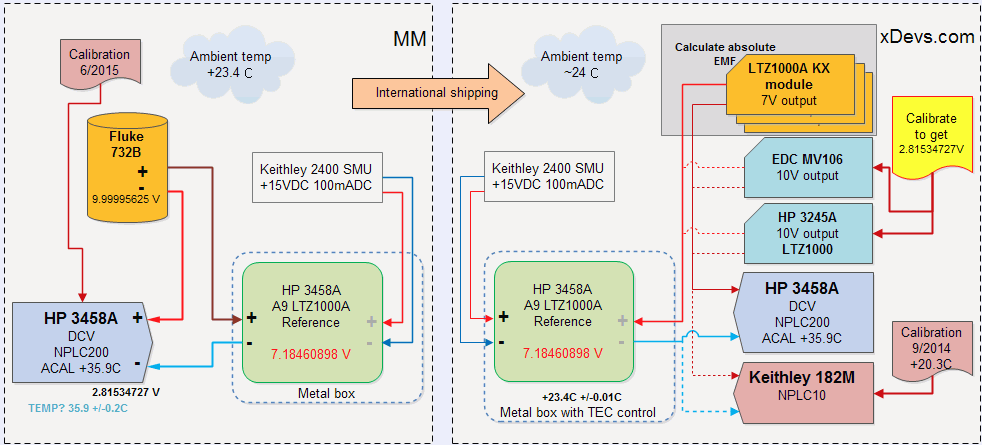
Image 75: Year 2016 xDevs USA-TW DC voltage transfer experiment
LTZ PCBA shipped from source location February 28, 2016 by regular USPS envelope mail. By no means this was reliable or robust enough transfer, so confidence was still quite low. There is a reason why commercial standards from Fluke, Wavetek and other big names in metrology are expensive and well rugged for travel/shipping. Shipping bare board even with high-end precision components is just asking for trouble due to mechanical, thermal and electrical stress induced to sensitive components.
Later experiment to transfer Volt/Ohm from USA lab was extended with personal visit for a week, with pair of Keithley 2002’s and set of small DIY standards as check-in luggage. Enough to say, I was almost late to the plane back to Taiwan, arrived at the gate just 20 minutes before departure. Fun times indeed.
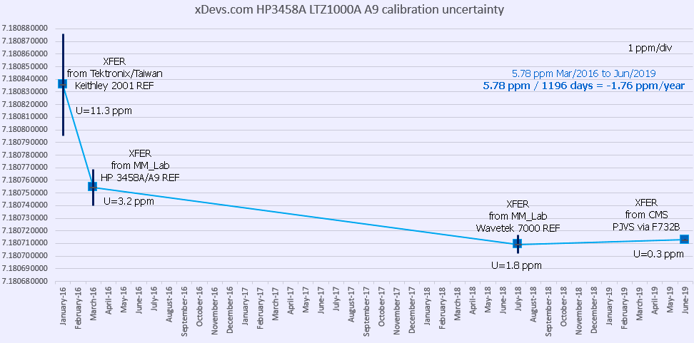
Image 76: Calibration uncertainty of xDevs TW Lab, DC voltage 10V
Transfer of the known +10V standard to DMMs such as 3458A or 5720A calibrator performed by executing routine calibration procedures, outlined in manufacturer’s service documentation. We keep logging of own DMMs LTZ1000A references and calibration constants, hence enabling the possibility to perform calibration adjustment of the instruments, without losing the history of the previous drift. Otherwise, adjustment of a precision instrument such as 8½ 3458A is not recommended, as this operation might easily bring a unit that was barely in specification well out of tolerance.
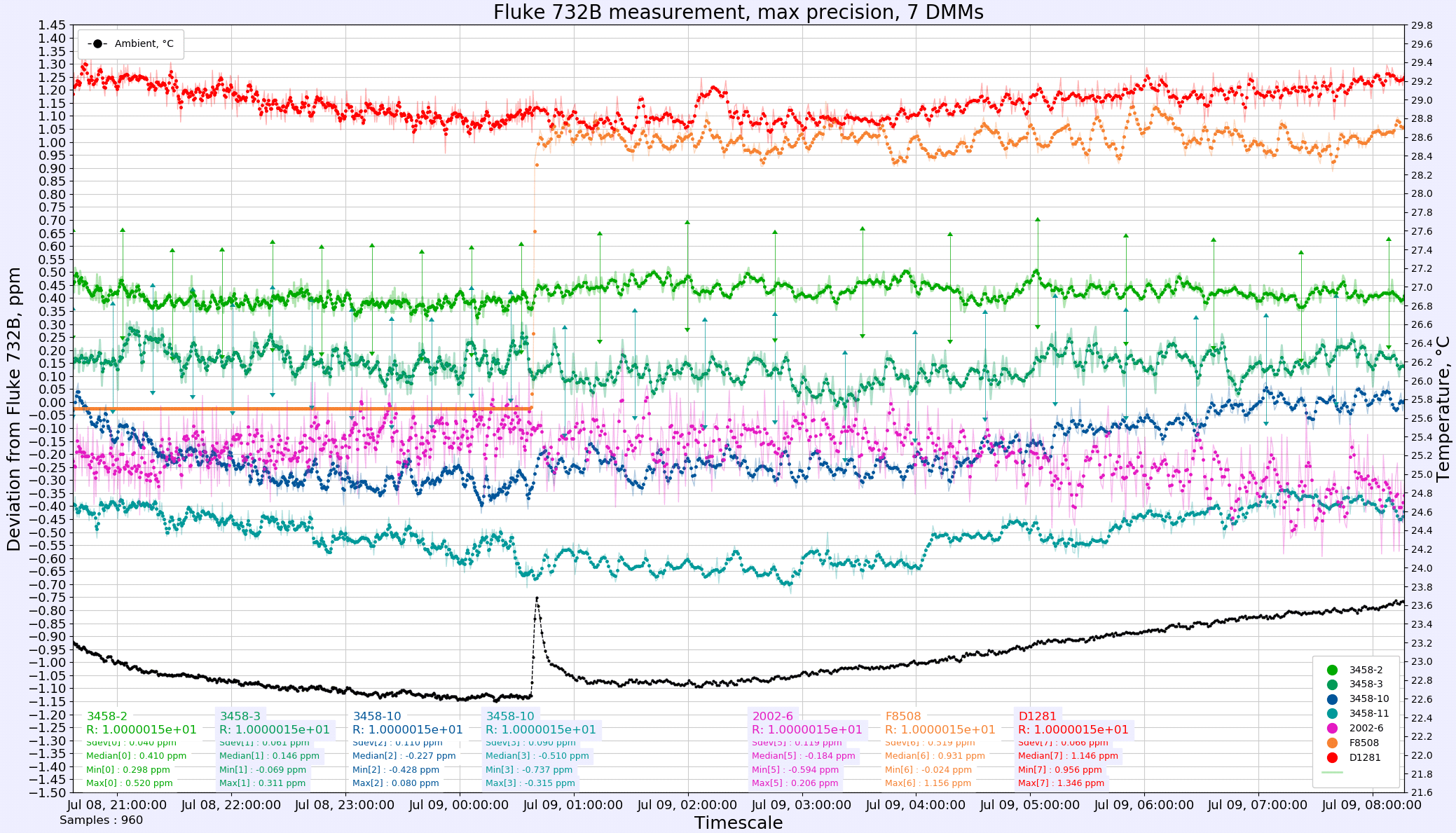
Image 77: Seven DMMs verifications from the calibrated Fluke 732B
Here on the chart all four 3458A are adjusted to the 732B value, while Keithley 2002, Fluke 8508A are kept with previous calibration constants. Datron 1281 DMM received few weeks ago, as the transfer meter from xDevs.com US Lab.
Transfer 10V to unknown Fluke/xDevs.com 792X “FX” reference
“FX” reference UUT output transferred from manual ratiometric measurement with Fluke 732B reference standard. The fixed range is used on the Keysight 3458A/X02 DMM as a detector. The following test uses 10-minute transfer specification with Fluke 732B output source as a reference. Gain was verified for stability ±0.05 ppm over the test period. Detector DC voltage offset is DUT is nulled prior to the measurement. Both standards powered by onboard batteries to avoid ground-loop risks.
| July 17, 2019 XFER, 732B=792X | Measurement | Uncertainty | Standard Deviation | REF / Δ |
|---|---|---|---|---|
| Transfer reference output | 10.0000152 VDC | 0.30 ppm | 0.300 ppm | |
| Reference measured output (+) | 10.00002061 VDC | 0.10 ppm | σ = 0.3847 µVDC | Δ = 0.537 ppm |
| Reference measured output (-) | -10.00001820 VDC | 0.10 ppm | σ = 0.3986 µVDC | Δ = 0.296 ppm |
| Reference calculated EMF | 10.00001940 VDC | 0.10 ppm | Δ = 0.416 ppm | |
| Detector zero offset | 0.00000002 VDC | |||
| UUT measured output (+) | 9.99998136 VDC | 0.10 ppm | σ = 0.3672 µVDC | |
| UUT measured output (-) | -9.99997966 VDC | 0.10 ppm | σ = 0.2748 µVDC | |
| Ratio positive polarity | .99999607 VDC | 0.20 ppm | ||
| Ratio negative polarity | .99999615 VDC | 0.20 ppm | ||
| UUT calculated output (+) | 9.99997599 VDC | 0.50 ppm | Δ = -0.036 ppm | |
| UUT calculated output (-) | -9.99997670 VDC | 0.50 ppm | Δ = 0.036 ppm | |
| UUT calculated EMF (Linear) | 9.99997634 VDC | 0.50 ppm | ||
| UUT calculated EMF (RSS) | 9.99997634 VDC | 0.36 ppm |
This transfer was completed July 17, 2019, with ambient temperature +24.0 °C, 24% RH, and 993.01 hPA pressure. Polarity reversal and standards reversal was performed manually with the use of low thermal EMF copper wires. Degree of freedom for measurements is 500. Stability of the 3458A DMM, in this case, matters only on short term (less than 1 hour) and our meters are proven to be far better than this.
xDevs.com/Fluke 792X standard is calibrated again the same day prior to transport to CMS Lab for its own PJVS calibration. It will be interesting to confirm traceable deviation of this 1:1 10V DC voltage transfer experiment, with the help of Keysight 3458A.
| Measurement data | Unit | Uncertainty | Std.deviation | Deviation | |
|---|---|---|---|---|---|
| xDevs.com Calibration date | August 1, 2019, before transport to CMS | ||||
| Transfer reference output | 10.0000152 | VDC | 0.300 ppm | ||
| 732B Reference measured output (+) | 10.0000230 | VDC | 0.100 ppm | σ = 0.217 µVDC | Δ = 0.776 ppm |
| 732B Reference measured output (-) | -10.0000207 | VDC | 0.100 ppm | σ = 0.199 µVDC | Δ = 0.548 ppm |
| Reference calculated +/- | 10.0000219 | VDC | 0.100 ppm | Δ = 0.662 ppm | |
| Detector zero offset | 0.0000006 | VDC | σ = 0.000000e+00 VDC | ||
| 792X UUT measured output (+) | 9.9999813 | VDC | 0.100 ppm | σ = 0.159 µVDC | |
| 792X UUT measured output (-) | -9.9999791 | VDC | 0.100 ppm | σ = 0.103 µVDC | |
| Ratio positive polarity | 0.99999583 | 0.200 ppm | |||
| Ratio negative polarity | 0.99999584 | 0.200 ppm | |||
| 792X UUT calculated output (+) | 9.9999735 | VDC | 0.500 ppm | Δ = -0.005 ppm | |
| 792X UUT calculated output (-) | -9.9999736 | VDC | 0.500 ppm | Δ = 0.005 ppm | |
| Temperature Δ | 0.14 | °C | 1.00 % | ±1.0 °C | |
| 792X UUT previous data | 9.9999779 | VDC | 0.600 ppm | ||
| Deviation from previous | -0.435 | ppm | 0.700 ppm | ||
| 792X UUT transfer result (Linear) | 9.9999735 | VDC | 0.500 ppm | ||
| 792X UUT transfer result (RSS) | 9.9999735 | VDC | 0.361 ppm |
Value deviation from previous July 17 test by -0.284 ppm, which is a bit much, but less than calculated uncertainty, so actual result could be better. Degree of freedom on this transfer equal 20.
This standard was trimmed to +10.000000 VDC according to our 3458A precisely when it was built on January 15, 2018, 555 days ago. Because extremely small transfer uncertainty the only way to prove above math is to perform traceable sub-ppm calibration for Fluke 792X reference directly. We will complete this task in August 2019 and perform a reverse transfer to 732B on the same day of standard return.
Transfer 10V to unknown 1.018V output of Fluke 732B
Three methods are used to perform a transfer from calibrated 10V output of our Fluke 732B to unknown 1.018 V output of the same reference. 1.018V is derived by the precision resistive divider. There is no output buffer amplifier on Fluke 732B 1.018V output, which produces a requirement for high-impedance detector to avoid loading errors. This output 1.018 V of the Fluke 732B reference is fixed and not user adjustable. Modern Fluke 732C provide 1.000 V and 100 mV outputs instead, as saturated voltage cells that have this voltage level are successfully replaced by solid-state references, reducing the importance of having 1.018 V stable output in the lab.
- Transfer method 1 : Use Keysight 3458A as a transfer device, using 10V transfer accuracy specifications
- Transfer method 2 : Use Fluke 8508A/001 and Datron 1281 in a ratiometric mode
- Transfer method 3 : Use Fluke 752A reference divider 1:10 and Keithley 155 null-meter
Correct measurements by all three methods should have a very good agreement to provide confidence in the selected transfer strategy.
Method 1 – Keysight 3458A DMM
For this method DMM will be used to measure set of voltage of known reference in both polarities and then measure unknown 1.018 V output in both polarities, and exactly same settings. Both measurements will be performed on fixed 10V range to benefit excellent INL performance of 3458A’s ADC. Results presented in Table.
| Parameter | Value | Uncertainty | Notes |
|---|---|---|---|
| Transfer standard VXFER | +10.0000152 V | 0.2 µV or 0.02 ppm | NMI Calibration report from May 31, 2019 |
| Measured 10V VREF output | +10.0000155 V | 1 µV or 0.10 ppm, σ = | 10 minute transfer accuracy spec |
| Measured 1.018V VUUT output | +1.0184215 V | 0.55 µV or 0.55 ppm, σ = | 10 minute transfer accuracy spec |
| Ratio of VUUT/VREF | +1.0184215 V | 0.55 ppm + 0.10 ppm | 10 minute transfer accuracy spec |
| EMF of VUUT | VXFER × Ratio = +1.018 V | 0.02 ppm + 0.65 ppm = 0.67 ppm Linear (0.65 ppm RSS) | Calculated positive EMF |
| Transfer standard VXFER | -10.0000152 V | 0.2 µV or 0.02 ppm | NMI Calibration report from May 31, 2019 |
| Measured 10V VREF output | -10.0000155 V | 1 µV or 0.10 ppm, σ = | 10 minute transfer accuracy spec |
| Measured 1.018V VUUT output | -1.0184215 V | 0.55 µV or 0.55 ppm, σ = | 10 minute transfer accuracy spec |
| Ratio of VUUT/VREF | -1.0184215 V | 0.55 ppm + 0.10 ppm | 10 minute transfer accuracy spec |
| EMF of VUUT | VXFER × Ratio = -1.018 V | 0.02 ppm + 0.65 ppm = 0.67 ppm Linear (0.65 ppm RSS) | Calculated negative EMF |
| Final result | (Vpos + -Vneg ) / 2 | 1.34 ppm Linear or 0.92 ppm RSS | Calculated with thermal EMF offset removed |
According to this measurement exercise once can assign the secondary output to be equal: +1.018 V ± 1.34 µV with 95% confidence. Transfer specification from Keysight 3458A specifications that are used in this example are reproduced in Table 4
| Range | Transfer accuracy, valid for 10 minutes | Note |
|---|---|---|
| 100 mV | 0.5 ppm of reading + 0.5 ppm of range | Fixed range measurements >4 min, Tambient ±0.5 °C, 10% to full-scale |
| 1 V | 0.3 ppm of reading + 0.1 ppm of range | |
| 10 V | 0.05 ppm of reading + 0.05 ppm of range | |
| 100 V | 0.5 ppm of reading + 0.1 ppm of range | |
| 1000 V | 1.5 ppm of reading + 0.05 ppm of range | Measurement within 5% of the initial value and following measurement settling |
Transfer of resistance, using calibrated 10.000 kΩ resistance standard
Similar math and concept apply for resistance as well. Resistance from transfer ESI SR104 calibrated with ±0.16 ppm uncertainty (9999.9995 Ω ±0.0016 Ω) accurate transfers of the reference can be made into lab standards, long-scale DMMs and Fluke 5720A calibrators. Unlike the case with DC Voltage, this can be done in longer time span, as most of old aged ESI SR104 have exceptional stability <0.1 ppm/year. Table below summarize overall stability between our available DC voltage sources and meters.
| Device | 24 hour specification | 90 day specification | 1 year specification |
|---|---|---|---|
| ESI SR104 | ± 0.5 ppm, maximum, <0.1 ppm typical | ||
| Fluke 742A | ± 2.5 ppm (180 day) | ± 4.0 ppm | |
| Fluke SL935 10K | < ±0.1 ppm (10 kΩ) | ± 0.8 ppm | ± 2.2 ppm |
| Fluke 5720A | ±2.0 ppm (10 kΩ) | ± 3.0 ppm | ± 4.0 ppm |
| Datron 1281 | ±1.6 ppm (20k range) / ± 0.4 ppm Ratio | ± 6.6 ppm | ± 6.6 ppm (w/Self-Cal) |
| Fluke 8508A/001 | ±1.5 ppm (19k range) / ± 0.5 ppm Ratio | ± 4.0 ppm | ± 7.5 ppm |
| Fluke 5450A | ±2.0 ppm (10 kΩ) | ± 3.5 ppm | ± 10.0 ppm |
| Fluke 8588A | ±2.0 ppm (20.2k range) / ± 1.21 ppm Ratio | ± 4.5 ppm | ± 7.5 ppm |
| HP 3458A | ±2.24 ppm (12k range) | ± 8.6 ppm | ± 10.6 ppm |
| Datron 4808 | ±2.5 ppm (10 kΩ) | ± 6.0 ppm | ± 15 ppm |
| Keithley 2002 | ±3.13 ppm (21k range) | ± 7.84 ppm | ± 9.84 ppm |
| Keithley DMM7510 | ±16.6 ppm (12V range) | ± 33.6 ppm | ± 33.6 ppm |
Table 1: Standards/DMM/MFC 10 kΩ stability over different calibration periods
SR104 calibration was transferred using the same procedure, with the help of three different DMMs, Keysight 3458A, Datron 1281 and Fluke 8508A/001.
Transfer from ESI SR104 10000 Ω to Fluke 5720/03/A calibrator working resistance output. Datron 1281 used as transfer detector, with DIY PTFE shielded cables connected to rear Channel A and Channel B ports. Electronic control with relays allows using Datron 1281 in a fully automated manner, reducing the chance of errors from cable chance and operator handling.
| Measurement | Unit | Uncertainty | Standard Deviation | Deviation | |
|---|---|---|---|---|---|
| Transfer date | July 24, 2019 | ||||
| Transfer reference output | 9999.9995 | Ω | 0.160 ppm | ||
| Reference measured output (+) | 10000.0085 | Ω | 0.300 ppm | σ = 64.872 mΩ | Δ = 0.900 ppm |
| Reference calculated +/- | 10000.0085 | Ω | 0.300 ppm | Δ = 0.900 ppm | |
| Detector zero offset | 0.0000 | Ω | σ = 1.000 mΩ | ||
| UUT measured output (+) | 9999.8200 | Ω | 0.300 ppm | σ = 18.816 mΩ | |
| Ratio | 0.99998115 | 0.600 ppm | |||
| UUT calculated output (+) | 9999.8110 | Ω | 0.760 ppm | Δ = +0.5 ppm (ACAL = 9999.806 Ω ±1.7 ppm) | |
| UUT calculated EMF (Linear) | 9999.8110 | Ω | 0.760 ppm | ||
| UUT calculated EMF (RSS) | 9999.8110 | Ω | 0.621 ppm |
Result for 10 KΩ agree very well, well below the 24-hour specification of Fluke 5720A calibrator.
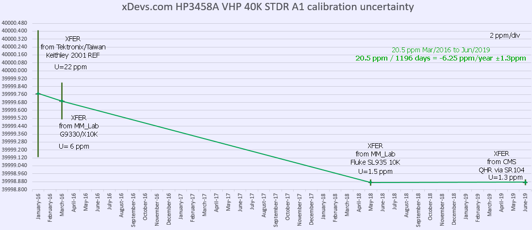
Artifact calibration verification of Keysight 3458A DMM tandem
Fluke 5720A/03 calibrator and precision Keysight 3458A 8½-digit DMMs are the main workhorses in our lab for many measurements. It is important to maintain accuracy and stability. With help of freshly calibrated 10 V, 10 kΩ and 1 Ω standards and ultra-linear ADCs in 3458A we can verify correct operation of ACAL functionality, that is vital for these instruments self-calibration ability.
We use no less than four 3458A together to improve confidence in measurements. Two meters are in constant 24/7 operation since 2016, and they have hardware modifications to improve stability. These two “golden standard” meters able to demonstrate linearity agreement on main 12VDC range better than ±0.05ppm and temperature stability better than 0.05 ppm/°C (without using ACAL).
To verify calibration, automated xDevs.com calkit python app was used to run thru various points, using Fluke calibrator as a precision source, and each of the DMMs as a device under test. Specifications for period 24 hours are used as limit levels.
Details about used equipment in this comparison:
- Fluke 5720A/03 multifunction 7½-digit calibrator, calibrated 7/24/2019 to SR104/732B/SL935-1
- Fluke 5725A amplifier, calibrated 7/24/2019 to SR104/732B/SL935-1
- 3 × 45 cm low-thermal spade lug cable set, equivalent to Fluke 5440A-7003
- 3458A unit, Keysight 3458A/001, reduced temperature, LTZ1000CH, <2ppm/year, calibrated 6/18/2019 to SR104/732B
- 3458B unit, Keysight 3458A/001, reduced temperature, LTZ1000ACH, <2ppm/year, modified DCI, calibrated 1/04/2017 to xDevs US Lab SR104/732B
- 3458C unit, Keysight 3458A/001/002 unmodified, calibrated 6/29/2019 to SR104/732B
- 3458D unit, Keysight 3458A/001 unmodified, calibrated 7/16/2019 to SR104/792X
- Python calkit application running on DE1-SoC FPGA board
- Agilent E5810A GPIB-LAN Gateway interface
DC Voltage function comparison
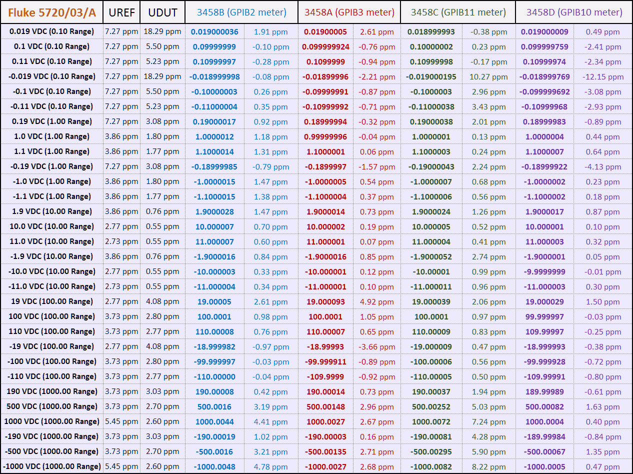
Each function range tested in both polarity, with 19%, 100% and 110% point, except 1kV range, which was tested at 19%, 50% and 100% point. All measurements are collected and combined MFC+DMM error from ideal value is calculated. Same test and procedure repeated for each DMM individually.
All measurements are taken with NPLC 100, AZERO ON after ACAL ALL, with floating DMM guard. Calibrator passed zero calibration shortly before each test run.
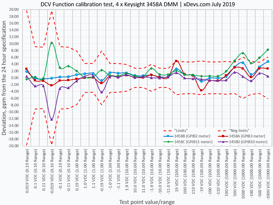
Data also presented as a graphical chart. Limits are calculated as RSS of MFC 24-hour specification and DMM 24-hour specification. This is overly strict test conditions because actual ACAL procedure on both 5720A and 3458A was NOT performed within the same 24-hour but on a much longer interval. We can see that few points on specific meters are slightly over the limits, such as +19 VDC, -19VDC on 100V range for 3458A (GPIB3) DMM and +500V, +1000V and -190V, -500V, -1000V for 3458C (GPIB11) DMM. Such test highlight the importance of using multiple DMMs to improve confidence on the actual lab capability. Even if one or two DMMs demonstrate worse accuracy, other meters can act as guardband providers on problematic tests.
Resistance function comparison
The same test repeated for resistance function, using 4-wire connection, DMM’s offset compensation function. Configuration of each meter was maintained same, and 100 &Omega – 100 kΩ ranges used OCOMP 1, DELAY 0.5 setting to mitigate cabling effects issues, as recommended by Keysight 3458A documentation.
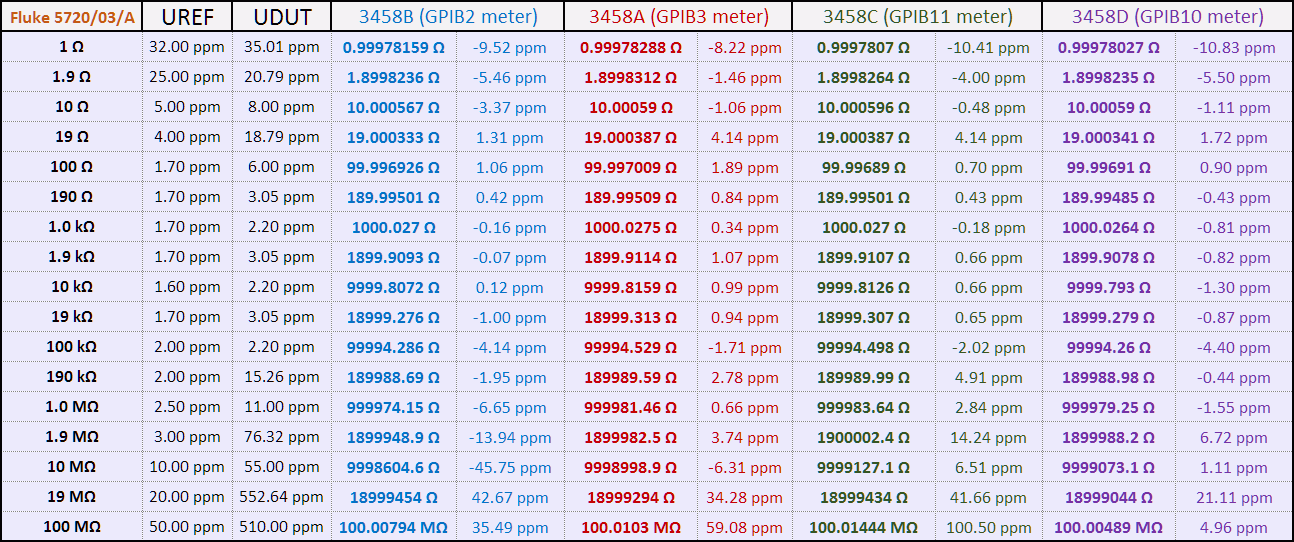
Each range was tested on 19% and 100% point, with reference resistance points provided from Fluke 5720A/03 calibrator. EXTSENSE is active on a calibrator, to enable the use of true 4-wire Kelvin connection to eliminate the impact of the cable resistance. Calibrator and DMM under test connected with 45 cm length Belden 8719 low-thermal copper spade lug cable set, similar to Fluke 5440A-7003.
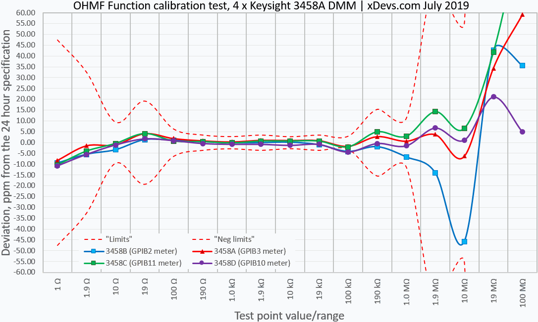
The graph reveals 100 kΩ point slightly towards low 24-hour specification limit, perhaps some more finetune is required for optimal settings. Currently, each point is sampled 30 times, and median of last 5 readings is taken as the final result. Other points reveal no issues, and system error for 100 Ω – 19 kΩ points is less than ±1.9 ppm, which is quite impressive.
AC Voltage function comparison
AC Voltage test is done in a similar manner, with test points:
- 10 mV to 750 V AC, with 1x and 3x steps.
- Same 45 cm Belden 8719 spade-lug cable set
- Frequency points 10 Hz, 20 Hz, 40 Hz, 100 Hz, 1 kHz, 10 kHz, 20 kHz, 50 kHz, 100 kHz, 300 kHz, 500 kHz, and 1 MHz
- 30 V tested with frequency up to 500 kHz
- 100 V tested with frequency up to 100 kHz
- 300 V tested from 100 kHz to 50 kHz, Fluke 5725A booster activated
- 750 V tested with points 100 Hz, 1 kHz, 10 kHz and 20 kHz, Fluke 5725A booster activated
Please click on the images to see full details on each item. Unlike other graphs, ACV test error represented in the percentage of the combined 5720A+3458A 24-specification.

Largest errors are contributed for frequency bandwidth over 50 kHz.
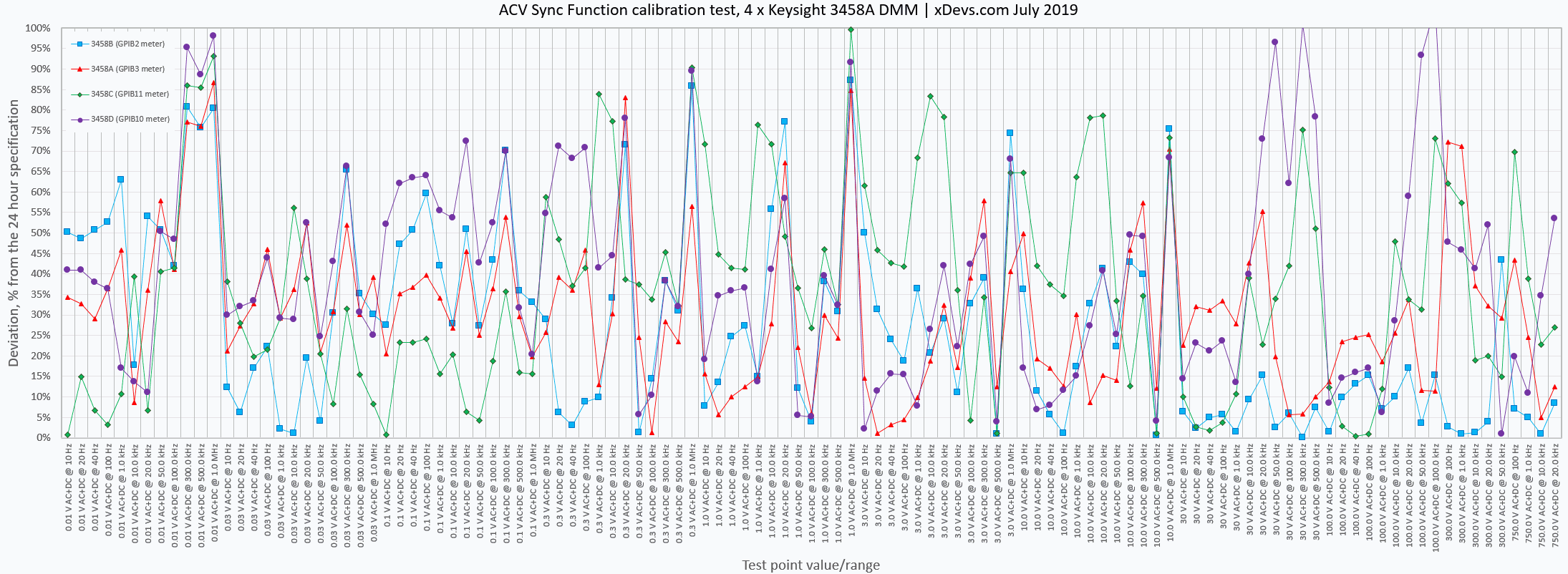
All 3458A’s configured with LFILTER ON, SETACV SYNC, DELAY 0, NRDGS 1, APER 0.6, RES 0.00001 command set. EXTSENSE is disabled on the calibrator for all points, only HI/LO connection is used.
DC Current function comparison
Current sourced from Fluke 5720A AUX output, with EXTGUARD disabled.
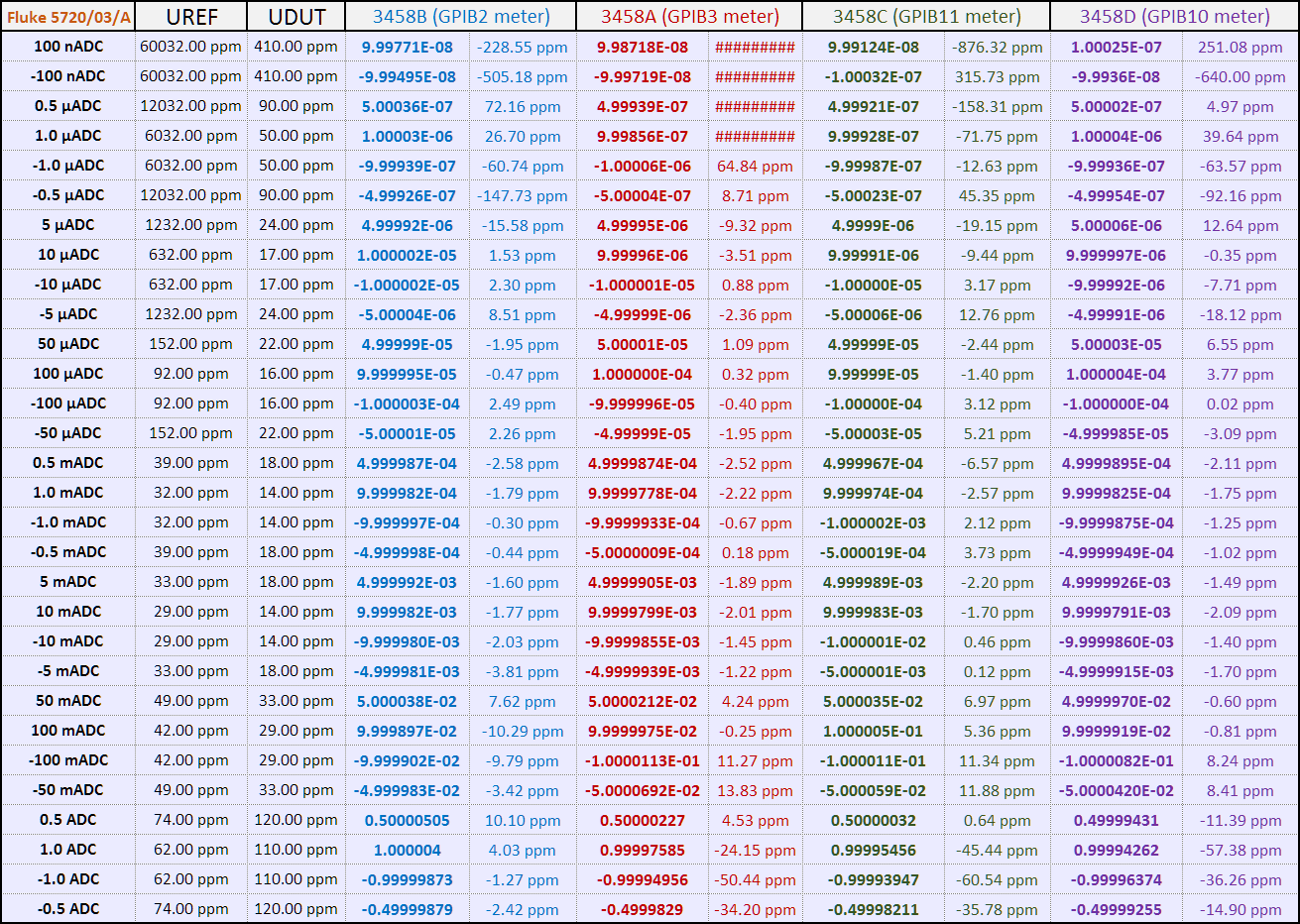
Each range was tested on 50% and 100% point in both polarity outputs. Calibrator and DMM under test connected with 45 cm length Belden 8719 low-thermal copper spade lug cable set, similar to Fluke 5440A-7003.
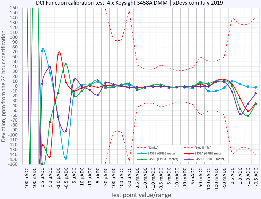
This test also clearly shows weak point, using calibrator to source currents below 100 µA due to noise floor limitation on lowest 220 µA current range. Using low-current source, such as Keithley 6430 would be better option for 3458A low current range verification.
AC Current function comparison
Now to answer the final question “Why one should ever need to maintain SI traceable accuracy for the lab?”. Annual uncertainty at even 2.0 ppm (0.0002%) already well below what most DMMs can achieve?
Such accuracy is important when we need to calibrate our 7½-digit calibrators or 8½-digit DMMs in-house on a periodic basis, often more frequent than once a year. Doing this externally would cost a fortune, so in fact, we performed this SI calibration to save cost. Establishing “xDevs Volt and xDevs Ohm” in long-term is actually cheaper to shipping high-end instruments such as Keysight 3458A to expensive external calibrations. 3458A’s calibration fee by Keysight Primary Standards Lab (which is also using JVS) is $2140 USD, shipping/handling excluded. Calibration for Fluke 5720A calibrator is even more expensive. Example cost breakdown is shown in Table 2.
| Instrument / Calibration service | Cost | Qty |
|---|---|---|
| Keysight 3458A/X02 | $2140 USD | 4 |
| Keithley 2002 | $1760 USD | 2 |
| Datron 1281 | $1500 USD | 1 |
| Fluke 5720A/5725A | $4900 USD | 1 |
| Shipping and handling, 120kg pallet | ~$1000 USD | 1 |
| Total one-time calibration cost | $17720 USD |
Only highest performance equipment is included in the list, however our lab has much more things that would need to be calibrated, such as AC transfer standards (Wavetek 4920, 4920M, Fluke 792A, TVC sets), SMUs and Electrometers, Keysight and Keithley nanovoltmeters, multiple resistance standards from Fluke, Guildline, L&N, resistance transfer standards like ESI SR1010/1030 series, ESI 242 bridges, etc. Also, some of our equipment is obsoleted a long time ago and special purpose, such as Keithley 1801 nanovolt amplifier and only a few commercial calibration labs have expertise about such things.
If we want to keep all these instruments calibrated externally and perform this service annually, the expense of keeping these instruments traceable and calibrated would be many times the cost of the instrument. Add the risk of damage, possible insurance costs, taxes and downtime in lab operation to get a better estimate, that high-end calibration can get very expensive fast, so only larger size business can afford to keep their instruments in best accuracy shape.
xDevs.com members are doing only non-profit research without external financing, so shipping all our precision equipment for external calibration is not a viable financial or logistic option. In this perspective investment into having in-house cardinal DC Voltage / Resistance standards and self-calibrating instruments such as Fluke 5720A, Fluke 752A, 720A, and Keysight 3458A DMMs provide a way to sustain high accuracy experimentation, with reduced financial effort. We will continue to maintain traceability to SI thru DC references and primary resistance standards in the future.
Livestream about calibration, metrology, and this article coverage
Summary and conclusion
ITRI CMS team and Dr. Shih-Fang Chen were very helpful during the calibration service, explained all the aspects in great detail and granted permission to publish and demonstrate how real National Measurement Lab is operating. It is amazing to see such advanced equipment in real life, as we see thousands of man-hours work put into results, invested by top-level international metrology research and engineering.
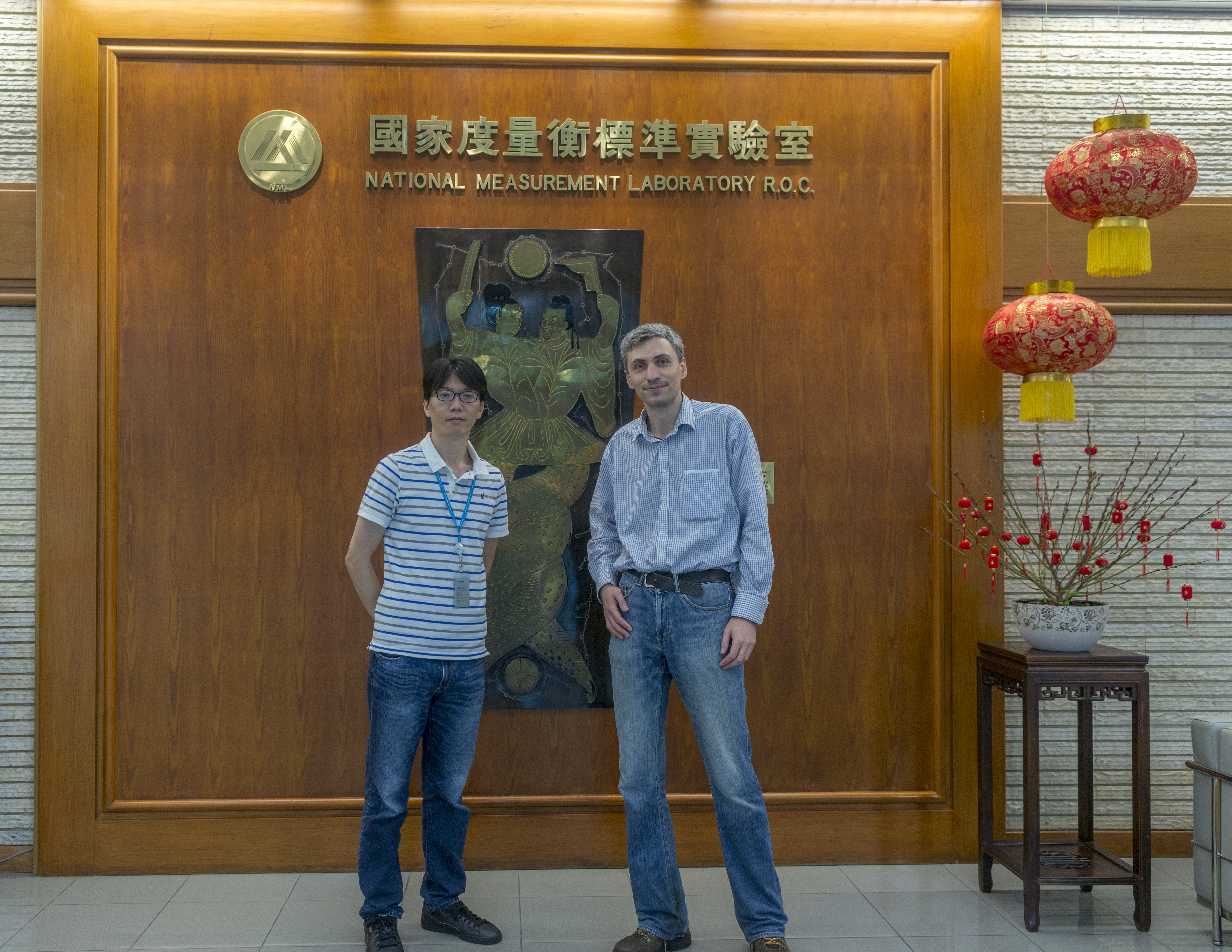
Image 78: Left to right: Dr.Shih-Fang Chen responsible for ITRI CMS Electrical Research Lab and Illya “TiN” Tsemenko, xDevs.com
This work and results would not be possible without the help of our readers and supporters, including donations and contributions. Special credits to go fellow USA Lab maintainer Todd M. and his decade-long efforts to keep the hobby-type lab in check for absolute accuracy. I have used his standards to perform transfers for Volt/Ohm during August 2016 meetup, and now with direct comparison to new SI Volt and Ohm, done by Taiwan’s NML CMS we see all that effort exceeded even our optimistic expectations.
Hopefully, this article can convince other metrology enthusiasts to reach out their nearest NMI to improve their own lab accuracy and have better confidence in measurements. Some may call all this serious case of volt-nuttery without any practical use. But I’d like to respectfully disagree, as the very device you use right now to read this electronic article is made possible because of advanced technology, made possible by a better understanding of physics and thousands of difficult measurements in process.
We wish to see more of such research, be it hobby level or science, helping to share and preserve complex knowledge about precision electronics and science of measurement in general, including repair or use of aged by still very capable secondary market instruments and references.
Modified: June 1, 2026, 11:22 p.m.
References
- Guildline QHR system page
- BIPM APMP.EM.BIPM-K11.5 protocol
- BIPM APMP.EM.BIPM-K11.3 comparison
- Wiki : Josephson Voltage Standard
- Hypres JVS System page
- Supracon AG : JVS Systems
- Industrial Technology Research Institute (ITRI) web-site
- ITRI NML CMS Electromagnetic lab site
- BIPM KCDB database
- Impact of Kelvin unit redefinition
- NIH: The Quantum Hall Effect in the Era of the New SI
- NIH : Historical publication "The Ampere and Electrical Standards"